Download
1 / 46
460 likes | 605 Vues
Department of Energy. Storm track response to Ocean Fronts in a global high-resolution climate model. R. Justin Small, Frank Bryan and Bob Tomas NCAR Young-Oh Kwon WHOI + 2 anonymous reviewers. Aims. Investigate influence of ocean fronts on atmospheric storm track in winter

E N D
Department of Energy Storm track response to Ocean Fronts in a global high-resolution climate model R. Justin Small, Frank Bryan and Bob Tomas NCAR Young-Oh Kwon WHOI + 2 anonymous reviewers
Aims • Investigate influence of ocean fronts on atmospheric storm track in winter • Surface storm track • Free-troposphere storm track • What are the key storm track statistics that are affected? • What affects baroclinicity? • Using a global atmospheric climate model • 1. North Atlantic • 2. Southern Ocean • 3. North Pacific
Experiments • Community Atmosphere Model version 4 • Developed at NCAR, Department of Energy, US labs • Hydrostatic, sigma-coordinate global model • ½ deg. grid spacing, 27 levels (<6 in lowest 1000m). • Twin experiments, atmosphere-only. • 1. Control has realistic SST in region (e.g. N. Atlantic) • 2. Smooth Global SST experiment • SST is a climatology based on satellite/in situ data (1/4deg., Reynolds et al 2007). • Each run for 60 years to gain some statistical significance.
Methods and Data • We use a high pass filter • V’=V-<V> • where <V> is 5-day mean at surface, seasonal mean or monthly mean in free troposphere • Compute climatological mean of quantities such as <V’V’> , <V’T’> • Apply smoothing to SST fields as boundary condition for AGCM. • 1 • 4000 passes of 1-4-1 filter • 1 • Comparisons are made with ERA-INTERIM data 1979-2009 (ERA-I) and OAFLUX, QSCAT
(b) (a) SMOOTH SST EXPERIMENT SST FOR CONTROL (c) (d) SST gradient difference SST DIFF SST difference C /100km North Atlantic case, Boreal winter (DJF).
Frequency distribution of strong SST gradients Low-res coupled model High-res coupled model Reynolds OI SST 1/4deg. Histograms of occurrence of binned SST gradients within 1deg. C/100km contour in North Atlantic including Gulf Stream. Uses data from DJF climatology. Units deg.C per 100km. Light smoothing of Reynolds OI SST 1/4deg. Heavy smoothing of Reynolds OI SST 1/4deg.
What storm track quantities are significantly affected by ocean front and what quantities are not?
(a) (b) Relative vorticity variability SMTH 10-6s-1 OAFLUX obs- Joyce and Kwon 2009 Std.dev(’) Smooth (c) (d) 10-5s-1 control 30% 10-6s-1 10-6s-1 Std.dev(’) Control Diff in Std.dev(’) +SST anomaly Standard deviation of near –surface transient eddy vorticity variability. Filtered to retain only timescales less than 5 days. Note that differences (control-smooth, bottom right panel) of std. dev (’) overly SST anomalies, and reach up to 30% of smooth value.
SMOOTH CONTROL hPa hPa Add significance DIFFERENCE hPa hPa SEA LEVEL PRESSURE VARIABILITTY. SLP sub-5day variability and differences
SMOOTH CONTROL 10-6s-1 10-6s-1 GEOSTROPHIC VORTICITY variability. DERIVED JUST FROM SLP. Surface geostrophic vorticity sub-5day variability and differences 25-30% DIFFERENCE 10-6s-1
Atlantic DJF: Meridional Heat Flux 30% V’T’ ERA-I V’T’ Control V’T’ Diffn. Control-Smooth V’T’ ERA-I ms-1K ms-1K ms-1K Transient eddy meridional heat flux 850hPa 25% Control-Smooth V’T’ ERA-I V’T’ Control V’T’ ms-1C ms-1K ms-1K ms-1K Transient eddy meridional heat flux 500hPa In the right panel only differences significant at 95% are shown, and contours show SST differences of +/- 2C from Fig. 1c. The number shown is the approx. ratio of the amplitude of the difference to the amplitude of the maximum in the smooth case, expressed as a percentage.
Atlantic DJF: Meridional wind variance 15% 7% std. dev V’V’ ERA-I V’V’ ERA-I V’V’ Control V’V’ Control-Smooth m2s-2 m2s-2 m2s-2 Transient eddy meridional wind variance 850hpa 10% V’V’ ERA-I Control-Smooth V’V’ Control V’V’ m2s-2 m2s-2 m2s-2 m2s-2 Transient eddy meridional wind variance 500hpa Low-light– CAM wind variance (& heat-flux) is too high compared to ERA-I and MERRA . Therefore adding the ocean front worsens the comparison.
BAROCLINICITY • WHAT COUNTERS THE EFFECT OF EDDIES IN REMOVING TEMPERATURE GRADIENT? • Latent heat release over western boundary currents helps maintain baroclinicity (Hoskins Valdes 1990,JAS) • Sensible heating maintains baroclinicity and anchors storm track (Nakamura et al 2008 GRL, Nonaka et al 2009, Sampe and Nakamura 2010 JCLIM, Ogawa et al 2012, Hotta and Nakamura 2011)
Baroclinicity (a) (b) (c) SMTH 950hPa ATL 50% (d) (e) (f) Baroclinicity SMTH 850hPa ATL 30% Eady (1949)- growth rate of most unstable mode Differences reduce to 7% at 500hPa
BOUNDARY LAYER HEAT BUDGET – HOR. ADVECTION VER. ADVECTION -d/dy V’T’ -d/dz W’T’ Thermodynamic potential temperature budget at 950hPa. Units degC./day. DJF climatology mean (from 10 years) sensible Heating Condensational Heating
FREE TROPOSPHERE HEAT BUDGET – Heat budget at 850hPa HOR. ADVECTION VER. ADVECTION -d/dy V’T’ -d/dz W’T’ Thermodynamic potential temperature budget at 850hPa. Units degC./day. DJF climatology mean (from 10 years) Condensational Heating sensible Heating
TRANSIENT EDDY HEAT FLUX DIVERGENCE – CONTROL BY OCEAN FRONT (a) (b) SMTH ATL (c) Vertically integrated total eddy heat flux divergence (color), for a) the SMTH case, b), ATL case and c) their difference. The corresponding climatological SST is shown as contours in a, b) and SST difference in c). SEE KWON AND JOYCE PRESENTATION
A few results from Southern Ocean focusing on South Indian Ocean.
(b) (a) V’T’ 850 DIFF SST DIFFERENCE 25%/83% ms-1K (c) (f) SST GRAD DIFF (SMOOTH) 33% BAROCLINICITY DIFF C /100km SOUTHERN OCEAN CASE, JJA. Relationship of transient eddy heat flux to SST gradient.
(a) SMTH CASE 10-5m2s-1 (b) CONTROL CASE 10-5m2s-1 SOUTHERN OCEAN CASE. Effective eddy diffusivity- eddy heat flux divided by mean temperature gradient
(a) (b) U950 MEAN SEA LEVL PRESSURE DIFF ms-1 hPa (c) (d) U950DIFF Z500 DIFF 20% reduction of zonal wind ms-1 gpm gpm Fig. 1. Circulation response in the North Atlantic in DJF. a, c, d) show diffeernce between the ATL and SMTH runs for a) The sea level pressure, c) the 950hPa zonal wind and d) 500hPa geopotential height. Here stipling denotes 95% significance according to the t-test. b) shows the climatological mean zonal wind at 950hPa in the SMTH case.
(a) U250 MEAN ms-1 (b) DIFF IN U250 INTERANNUAL STANDARD DEVIATION 30% ms-1 Fig. 2. a) The climatological mean 250hpa zonal wind (U250) in the SMTH case for DJF over the North Atlantic. B) the difference in standard deviation of U250 between ATL and SMTH run. Stipling in b) denotes 95% significance according to the f-test.
Conclusions • Ocean fronts induce large (~30%) changes in heat flux, moisture flux (~40%), and precip. in winter • Reaching well above the boundary layer – to > 500hPa • vorticity variance at surface (~30%) • Smaller influence on wind (~10%) and sea level pressure (few% locally) variance • Baroclinicity and eddy heat flux • Maintained by sensible heating in boundary layer • Condensational heating above that • In Southern ocean v’T’~ dT/dy • Results may be (very) model-dependent
Heat budget at 850hPa – diff unsmoothed minus smoothed HOR. ADVECTION VER. ADVECTION -d/dy V’T’ -d/dz W’T’ sensible Heating Condensational Heating
(a) (b) (b) (c) Sens. Ht. dT/dt 950hPa T 950hPa Kday-1 Wm-2 (f) (d) (e) T850 diff. Lat. Ht. dT/dt 850hPa T 850hPa Wm-2 Kday-1 (h) (i) (g) dT/dt 500hPa T 500hPa Total Prec. mmday-1 Kday-1 Fig. 14. Surface heating and tropospheric temperature differences between ATL and SMTH run. a, d, g) show surface sensible heating, surface latent heating, and precipitation respectively. b), e, and h) show temperature tendency at 950hPa (from sensible heat), and 850hPa and 500hPa (from condensational heating.) c), f), and I) show the corresponding air potential temperature. In right panels the corresponding SST anomalies of +2C(-2C) are shown as thick (thin) solid lines.
Methods ERA-INTERIM “heat flux” V’T’ for DJF for different frequency bands ERA, 5 day ERA, 30 day ERA, 90 day ms-1K ms-1K ms-1K
Frequency response 25deg.
Discussion • Results get slightly shaky from here on…
(a) To-2 (b) To- Strong baroclinicity Weak baroclinicity T’=4 T’=2 To+2 To+ Noting that v’T’ ~ baroclinicity (T) leads to possible: Mechanism 1. Mixing length. Figure 17. Schematic showing scenarios for increases to v’T’ due to an ocean front. The solid lines are hypothetical isotherms deliniating a kink in a baroclinic zone (developing into a cold and warm front.) In a), b) there is no notable change to the displacement of the isotherm (no change to v’)
Strong baroclinicity (c) t=t1 t=t2 t=t0 (d) Weak baroclinicity t=t0 t=t2 t=t1 Eady growth rate would suggest… Mechanism 2. growth rate ~ T Figure 17. Schematic showing possible scenarios for increases to v’T’ due to an ocean front. The solid lines are hypothetical isotherms deliniating a kink in a baroclinic zone (developing into a cold and warm front.) In c), d) there is a notable change to the displacement of the isotherm (change to v’). In c, d) a stronger baroclinicity leads to larger growth rate and displacements leads to larger changes in v’T’, particularly later in wave development.
SMTH ATL ATL hPa hPa Add significance hPa hPa Sea Level Pressure sub-5day variability and differences
11% ms-1 ALL GEOSTROPHIC Surface geostrophic V sub-5day differences 30% 10-5s-1 Surface geostrophic vorticity sub-5day differences
Comparison with Aquaplanet C per 100km Nakumura, Sampe et al. 2008, Sampe et al. 2010. Maximum SST gradient changed by factor ~6 in zonal mean. SST anomalies 5C or more (all one-sign) in zonal mean. SMOOTH CONTROL C /100km C /100km Maximum SST gradient changed by factor ~3 locally (smaller in zonal mean). SST anomalies up to 5C locally, more typically 2C or less and have both signs.
Conclusions • Ocean fronts induce large (~30%) changes in heat flux, moisture flux (~40%), vorticity variance, and precipitation in winter • Reaching well above the boundary layer – to > 500hPa • Smaller influence on wind (~10%) and sea level pressure (few% locally) variance • Comparison with reanalysis: • Model Heat flux agrees well with ERA-I and MERRA in Atlantic, is too high in Southern Ocean • Model wind variance is too high in both regions • Results may be (very) model-dependent
Way ahead Moving to CAM-5, high-resolution • Improved convection schemes etc. • ¼ deg, 30 levels • maybe 1/8deg, more vertical levels Coupled simulations • ocean model 1/10th deg. Parallel Ocean Program (POP) • 40+ years so far Spatial filtering on-line in model coupler (for SST, fluxes etc.) Show animation (if audience still awake)
Do ocean fronts influence storm tracks? • Strong influence • Latent heat release over western boundary currents helps maintain baroclinicity (Hoskins Valdes 1990) • Ocean fronts essential to eddy variability associated with polar front jet (Nakamura et al 2008) • Moderate Influence • Ocean dynamics shifts location of storm track (Wilson et al. 2009, Brayshaw et al. 2011) • No influence • Self-maintenance, eddies and mean jet, no role of ocean (Robinson 2006)
CAM model Courtesy Joe Tribbia, NCAR
Gulf Stream and atmospheric convection CCSM. From Bryan et al 2010. FIG. 4. Laplacian of sea level pressure (color, 1029 Pa m22) and horizontal convergence of lowest model level wind (contours, interval 2 3 1026 s21, negative values dashed) for the winter season (Nov-Feb) in the Gulf Stream region: high-res CCSM4. From Minobe et al 2008. Low level convergence proportional to Laplacian of sea level pressure and to Laplacian of SST.
Vertically integrated total eddy heat flux divergence Meridional component only i.e. d/dy v’T’ etc
Atlantic DJF: 850hPa Transient eddy “heat flux” 30% V’T’ ERA-I V’T’ Control V’T’ Diffn. V’T’ ERA-I Control-Smooth ms-1K ms-1K ms-1K Transient eddy meridional wind variance 15% 7% std. dev V’V’ ERA-I V’V’ ERA-I V’V’ Control V’V’ Control-Smooth m2s-2 m2s-2 m2s-2 In the right panel only differences significant at 95% are shown, and contours show SST differences of +/- 2C from Fig. 1c. The number shown is the approx. ratio of the amplitude of the difference to the amplitude of the maximum in the smooth case, expressed as a percentage.
Atlantic DJF: 500hPa Transient eddy “heat flux” 25% Control-Smooth V’T’ ERA-I V’T’ Control V’T’ ms-1C ms-1K ms-1K ms-1K Transient eddy meridional wind variance 10% V’V’ ERA-I Control-Smooth V’V’ Control V’V’ m2s-2 m2s-2 m2s-2 m2s-2 Low-light– CAM wind variance (& heat-flux) is too high compared to ERA-I and MERRA . Therefore adding the ocean front worsens the comparison.
Indian Ocean JJA: 850hPa Transient eddy “heat flux” V’T’ ERA-I V’T’ Control V’T’ Diffn. 30% ms-1K ms-1K ms-1K ms-1K ms-1K Transient eddy meridional wind variance V’V’ ERA-I V’V’ Diff’n V’V’ Control 14% m2s-2 m2s-2 m2s-2 In the right panel only differences significant at 95% are shown, and contours show SST differences of +/- 2C from Fig. 1c. The number shown is the approx. ratio of the amplitude of the difference to the amplitude of the maximum in the smooth case, expressed as a percentage. Low-light– CAM wind variance (& heat-flux) is too high compared to ERA-I and MERRA . Therefore adding the ocean front worsens the comparison.
Indian Ocean JJA: 500hPa Transient eddy “heat flux” V’T’ ERA-I V’T’ Control V’T’ ERA-I 25% ms-1K ms-1K ms-1K Transient eddy meridional wind variance V’V’ ERA-I V’V’ Diff’n V’V’ Control 15% m2s-2 m2s-2 m2s-2 In the right panel only differences significant at 95% are shown, and contours show SST differences of +/- 2C from Fig. 1c. The number shown is the approx. ratio of the amplitude of the difference to the amplitude of the maximum in the smooth case, expressed as a percentage.