Download
1 / 8
80 likes | 187 Vues
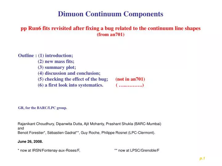
Dimuon Continuum Components pp Run6 fits revisited after fixing a bug related to the continuum line shapes (from an701). Outline : (1) introduction; (2) new mass fits; (3) summary plot; (4) discussion and conclusion;

E N D
Dimuon Continuum Components pp Run6 fits revisited after fixing a bug related to the continuum line shapes (from an701) Outline : (1) introduction; (2) new mass fits; (3) summary plot; (4) discussion and conclusion; (5) checking the effect of the bug; (not in an701) (6) a first look into systematics. ( …..……….) GR, for the BARC/LPC group. Rajanikant Choudhury, Dipanwita Dutta, Ajit Mohanty, Prashant Shukla (BARC-Mumbai) and Benoit Forestier*, Sébastien Gadrat**, Guy Roche, Philippe Rosnet (LPC-Clermont). June 26, 2008. * now at IRSN/Fontenay-aux-Roses/F, ** now at LPSC/Grenoble/F p.1
(1) introduction. The resonance line shapes had been normalized prior to being used in the fits when the smeared gaussian functional was introduced as the resonance line shape about one year ago. Sadly enough, forgot to do it for the continuum line shapes functionals. The problem was discovered when Yasuyuki Akiba asked me to provide DY yields for mass cuts at 3 or 4 GeV following the presentation at the HL on April 10. Then, realized the continuum components numbers in the fit panel were not the same as the integral of the corresponding line shape functions. The numbers were as follows: North arm, variable binning mass>2 GeV NDY = 173 (integral) 220 +/- 295 (fit panel) 3 96 4 50 North arm, uniform binning mass>2 GeV NDY = 83 (integral) 105 +/- 167 (fit panel) 3 46 4 24 Normalizing all continuum line shape functionals fixed the problem and all pp Run6 fits were redone (pp Run5 fits were not because of lower data statistics, and are not shown any more). Two pp Run6 mass fits are given in the following slides and submitted for preliminary approval. A summary of all new fits is given in a fourth slide before the conclusion, followed by checks of the effect of the bug.. The systematics section was added for the LLR presentation on 06/26/2008 See an701 for details. p.2
(2) new mass fits. North pp Run6. option I being used, LL not suitable Very low probability resulting from both the data points at low mass, below the J/, and the dispersion of points at all mass. Notice the DY number in the fit panel is the same as the integral number in the previous slide (173). submitted for preliminary approval(?) p.3
South pp Run6. option I being used, LL not suitable Much better probability now. submitted for preliminary approval p.4
(3) summary plot. J/ yields and other components ratios to J/ from the various mass fits. From left to right, the red points are from Run 6 North no pt cut and pt<3 GeV/c, the blue points from Run 6 South no pt cut and pt<3 GeV/c, and the aqua points from Run 6 North and South, uniform binning. The triangle points are those submitted for preliminary approval. One observes some dispersion of points, beyond statistics, especially for BB, where the first and last points get far off. The North and South plots submitted for preliminary approval are slightly off in regard to statistical errors (for BB). The same line shape functions have been used for both arms. One might consider to double check for any North vs. South difference in line shapes with the simulated data we presently have (limited statistics though) and/or include the observed discrepancy within systematics errors. p.5
(4) discussion and conclusion. (straight from an701) The resonance line shapes are already very well defined, especially for J/. The extracted ’ yield agrees with the COM value of 1.73 +/- 0.23 % of the J/ yield (cf. Sébastien Gadrat’s thesis, p. 121). The Υ yield from the Run 6 data seems to be well assessed, 0.14 +/- 0.05 % of J/’s. The continuum components line shapes current simulation suffers from limited statistics. This is even worse for pt shapes as we used the only full mass range files. More statistics is already available and more will be generated in the near future. However, a comparison of the new and old frameworks line shapes, the old ones being produced with high statistics, does not show large differences, except at the high mass tails. Thus, we infer our current shapes are not far off. The continuum components yields are sensitive to combinatorial background subtraction, especially at low mass, which could be an issue. Our comparison of event mixing and like-sign subtraction for the pp Run 5 data indicates both open charm yields are not consistent, but both open beauty yields are, within large errors though. Notice also event mixing does not reproduce like-sign distributions. We’ll try event mixing later on, and again, infer our current open beauty yields should not be far off. Pythia generated pt shapes are definitely not consistent with data pt shapes for values above 3 GeV/c. However, that does not affect the open beauty yield relative to J/’s. We’ll try other event generator later on, when they get available. There is a positive argument though, that we get the right ’ yield, a weak signal, also sensitive to background subtraction. Thus, as a final conclusion, we’d like to claim a first observation of beauty production in the dimuon channel in pp at 200 GeV, Drell-Yan being consistent with zero within errors. The plot(s) in slide(s) (3 and) 4 are submitted for preliminary approval. p.6
(5) checking the effect of the bug. The points before bug correction are shown as open figures. Except for DD where one can notice large differences, all other components were not that much affected. Remember the resonance line shape functionals were normalized prior to being used in the fits, thus the J/ numbers stay identical or very close to, while the weaker resonance numbers (’ and Υ) show some fluctuation, still staying well within errors, especially for ’. p.7
(6) a first look into systematics. In our analysis, we would assume two main systematics origins : (1) the line shape functionals and parameters (keeping in mind Pythia is the event generator), and (2) the data background subtraction, presently like sign subtraction. We are presenting (1). The blue triangle points are the reference ones, same as in the previous slide, all nominal parameters values. The solid square points are nominal + sigma, and open square nominal – sigma; - red points, all BB, DY, DD components involved; - blue points, BB only involved, pink points DY only, aqua points DD only. Clearly, the effect of the BB parameters is most important, DY and DD being with no much effect. Notice the large differences in probability due to the BB change in parameters. Concerning open beauty we are mostly interested in, the yield in % of J/ in South can be taken as 23.3 +/- 5.3 stat (triange point) +/- 11.0 syst (extreme points) p.8