Graphs

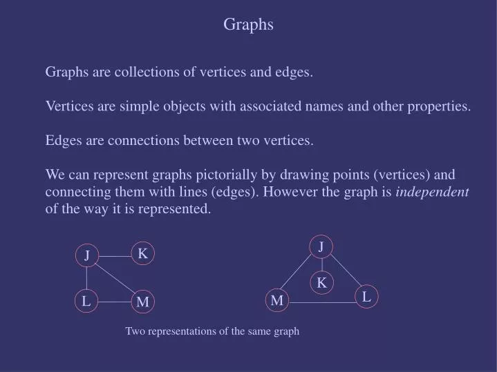
1. Graphs Graphs are collections of vertices and edges. Vertices are simple objects with associated names and other properties. Edges are connections between two vertices. We can represent graphs pictorially by drawing points (vertices) and connecting them with lines (edges). However the graph is independent of the way it is represented. J K J K L M L M Two representations of the same graph

2. A H I G B C K J D E L M F Paths A path is a list of vertices in which successive vertices are connected by edges in a graph. Example: BAFEG is a path.

3. A H I G B C K J D E F L M Connected Graphs A graph is connected if there is a path from every node to every other node in the graph1. A graph that is not connected is made up of connected components. The graph below has three connected components. 1 Intuitively, if the vertices were physical objects and the edges were strings connecting them, a connected graph would stay in one piece if picked up by any vertex.

4. H I K J L M Paths and Cycles A simple path is a path in which no vertex is repeated. Examples: BAFE is a simple path. BAFEGAC is not a simple path A cycle is a simple path except that the first and last vertex are the same (a path from a point back to itself). Example: AFEGA is a cycle. A G B C D E F

5. H I Trees and Forests A graph with no cycles is called a tree. A group of disconnected trees is called a forest. The figure below represents a forest of three disconnected trees. A K G J B C D L M E F

6. Spanning Trees A spanning tree of a graph is a subgraph that contains all the vertices but only enough of the edges to form a tree. The figure below shows a graph (left) and one of its possible spanning trees (right). A A G G B C B C D D E E F F

7. Spanning Trees If we add any edge to a spanning tree, it must form a cycle (since there is already a path between the two vertices that it connects). A tree with V vertices has exactly V-1 edges. If a tree has less than V-1 edges, it can't be connected. If it has more than V-1 edges, it must have a cycle. (But if it has exactly V-1 edges it need not be a tree!). A A G B C G B C D D E E F F

8. Sparse and Complete Graphs V: number of vertices E: number of edges E can range anywhere between 0 and 1/2(V)(V-1) Graphs with all edges present are called complete graphs. Graphs with relatively few edges (say less than VlogV) are called sparse. Graphs with relatively few of the possible edges missing are called dense. K K J K J J L M L M L M Sparse Complete Dense

9. Directed, Undirected, and Weighted Graphs So far we've dealt with undirected graphs, the simplest type. In weighted graphs, integers (weights) are assigned to each edge to represent, say, distances or costs. In directed graphs, edges are “one-way”: an edge may go from J to K but not from K to J. Directed weighted graphs are sometimes called networks. 2 2 K K J K J J 6 3 1 3 1 4 4 5 L M L M L M 7 Directed Directed weighted (network) Weighted

10. Graph Representation We will look at two data structure representations of graphs. • Adjacency matrix representation • Adjacency structure representation Usually, the choice of representation depends on whether the graph in question is dense or sparse, however this also depends on the nature of the operations to be performed as well. The first step is to map the vertex names to integers. This is to allow accessing vertex information through an array index. Throughout, we will assume the existance of a function index which, when called with a vertex name, returns the integer representation of that vertex. We will also assume the existance of a function name which when called with a vertex index, returns the vertex name. In the examples to follow, we map vertices with single-character names to integers.

11. A G B C D E F Adjacency Matrix Representation This representation is suitable for dense graphs. A VxV array a of boolean values is maintained, with a[x,y] set to true if there is an edge from vertex x to vertex y and false otherwise. Each edge is represented by two bits: a[x,y] and a[y,x]. Obviously this is a symmetric matrix and even though we could store only half of it, it is inconvenient to do so from an indexing viewpoint. Note that it is usually convenient to assume that there's an “edge” from each vertex to itself, so a[x,x] is set to true. (In some cases, it is more convenient to set the diagonal elements to false.)

12. A G B C D E F Adjacency Structure Representation This representation is suitable for sparse graphs. All vertices connected to each vertex are listed on an adjacency list for that vertex. This can be easily done with linked lists. Note that final outcome of adjacency lists depend on how the edges were input. For example, for adjacency list for ‘A’ above, the input edges were AG, AC, AB, AF.

13. Constructing Adjacency Lists #include <iostream> using namespace std; const int maxV = 1000; typedef struct node { int v; node* next; } node, *nodePtr; nodePtr z = 0; int V=0, E=0; // vertex and edge count nodePtr adj[maxV]; // adjacency list int index(int i) { return i; }

14. void load() { int j, x, y; nodePtr t; int v1, v2; // can be other types. see 'index' cin >> V; // get number of vertices cin >> E; // get number of edges cout << V << " vertices, " << E << " edges." << endl; z = new(node); z->next = z; // init lists for (j=0; j<V; j++) adj[j] = z; // read edges for (j=0; j<E; j++) { cin >> v1; cin >> v2; // get edge vertices x = index(v1); y = index(v2); cout << "Edge " << j << ": " << x << ", " << y << endl; t = new node; t->v = x; t->next = adj[y]; adj[y] = t; t = new node; t->v = y; t->next = adj[x]; adj[x] = t; } } Constructing Adjacency Lists

15. void list() { int i; nodePtr t; for (i=0; i<V; i++) { t = adj[i]; if (t != z) cout << i << " connected to "; while (t != z) { cout << t->v << ((t->next == z) ? " " : ", "); t = t->next; } cout << endl; } } Constructing Adjacency Lists

16. Depth-First Search When dealing with graphs, many questions can arise: Is the graph connected? If not, what are its connected components? Does the graph have a cycle? To answer these kinds of questions, depth-first search is used.

17. Depth-First Search void dfs() { int id=0, k; int val[maxV]; for (k=0; k<V; k++) val[k] = 0; for (k=0; k<V; k++) if (!val[k]) visit(val, k, id); }

18. Depth-First Search void visit(int* val, int k, int & id) { nodePtr t; cout << "visit: visiting node " << k << endl; val[k] = ++id; t = adj[k]; while (t != z) { if (val[t->v] == 0) visit(val, t->v, id); t = t->next; } }

19. Depth-First Search DFS for a graph represented with adjacency lists requires time proportional to V + E. We set each of the V val values (hence the V term) and we examine each edge twice (hence the E term). DFS for a graph represented with an adjacency matrix require time proprotional to V2 (every bit in the matrix is checked).

20. Non-Recursive Depth-First Search We can implement DFS non-recursively. We simply replace the frame stack with our own stack structure. Our dfs() function two slides back remains almost the same, however the function visit() is now made non-recursive. void dfs() { int id=0, k; int val[maxV]; // stack_init() // initialize the stack for (k=0; k<V; k++) val[k] = 0; for (k=0; k<V; k++) if (!val[k]) visit(val, k, id); }

21. Non-recursive Depth-First Search void visit(int* val, int k, int & id) { nodePtr t; cout << "visit: visiting node " << k << endl; stack_push(k); do { k = stack_pop(); val[k] = ++id; t = adj[k]; while (t != z) { if (val[t->v] == 0) { stack_push(t->v); val[t->v] = -1; } t = t->next; } } while (! Stackempty()); }

22. Breadth-First Search Rather than use a stack to hold vertices, as in DFS, here we use a queue. This leads to a second way of graph traversal, known as breadth-first search. To implement BFS, simply change stack operations to queue operations. Changing the data structure this way affects the order in which the nodes are visited.

23. DFS v. BFS In terms of vertex exploration, how do you think DFS and BFS differ? DFS: Explore deeper into the graph frontier (process closer vertices only after farther-away vertices have been explored). BFS: Sweep around starting point, exploring deeper only after all surrounding vertices in vicinity have been explored Order of traversal in either method is highly dependent on the order in which the vertices appear in the adjacency lists.