Download
1 / 20
290 likes | 1.26k Vues
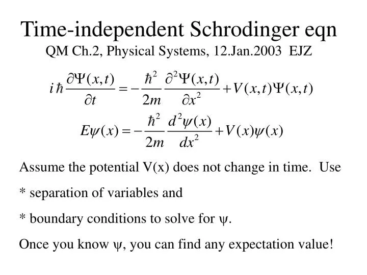
Time-independent Schrodinger eqn QM Ch.2, Physical Systems, 12.Jan.2003 EJZ. Assume the potential V(x) does not change in time. Use * separation of variables and * boundary conditions to solve for y . Once you know y , you can find any expectation value!. Outline:.

E N D
Time-independent Schrodinger eqnQM Ch.2, Physical Systems, 12.Jan.2003 EJZ Assume the potential V(x) does not change in time. Use * separation of variables and * boundary conditions to solve for y. Once you know y, you can find any expectation value!
Outline: • “Derive” Schroedinger Eqn (SE) • Stationary states • ML1 by Don and Jason R, Problem #2.2 • Infinite square well • Harmonic oscillator, Problem #2.13 • ML2 by Jason Wall and Andy, Problem #2.14 • Free particle and finite square well • Summary
Stationary States - introduction If evolving wavefunction Y(x,t) = y(x) f(t) can be separated, then the time-dependent term satisfies (ML1 will show - class solve for f) Separable solutions are stationary states...
Separable solutions: (1) are stationary states, because * probability density is independent of time [2.7] * therefore, expectation values do not change (2) have definite total energy, since the Hamiltonian is sharply localized: [2.13] (3) yi = eigenfunctions corresponding to each allowed energy eigenvalue Ei. General solution to SE is [2.14]
ML1: Stationary states are separable Guess that SE has separable solutions Y(x,t) = y(x) f(t) sub into SE=Schrodinger Eqn Divide by yf: LHS(t) = RHS(x) = constant=E. Now solve each side: You already found solution to LHS: f(t)=_________ RHS solution depends on the form of the potential V(x).
Now solve for y(x) for various V(x) Strategy: * draw a diagram * write down boundary conditions (BC) * think about what form of y(x) will fit the potential * find the wavenumbers kn=2 p/l * find the allowed energies En * sub k into y(x) and normalize to find the amplitude A * Now you know everything about a QM system in this potential, and you can calculate for any expectation value
Square well: V(0<x<a) = 0, V= outside What is probability of finding particle outside? Inside: SE becomes * Solve this simple diffeq, using E=p2/2m, * y(x) =A sin kx + B cos kx: apply BC to find A and B * Draw wavefunctions, find wavenumbers: kn a= np * find the allowed energies: * sub k into y(x) and normalize: * Finally, the wavefunction is
Square well: homework 2.4: Repeat the process above, but center the infinite square well of width a about the point x=0. Preview: discuss similarities and differences
Ex: Harmonic oscillator: V(x) =1/2 kx2 • Tipler’s approach: Verify that y0=A0e-ax^2 is a solution • Analytic approach (2.3.2): rewrite SE diffeq and solve • Algebraic method (2.3.1): ladder operators
HO analytically: solve the diffeq directly Rewrite SE using * At large x~x, has solutions * Guess series solution h(x) * Consider normalization and BC to find that hn=an Hn(x) where Hn(x) are Hermite polynomials * The ground state solution y0 is the same as Tipler’s * Higher states can be constructed with ladder operators
HO algebraically: use a± to get yn Ladder operators a±generate higher-energy wave-functions from the ground state y0. Work through Section 2.3.1 together Result: Practice on Problem 2.13
Ex: Free particle: V=0 • Looks easy, but we need Fourier series • If it has a definite energy, it isn’t normalizable! • No stationary states for free particles • Wave function’s vg = 2 vp, consistent with classical particle: check this.
Finite square well: V=0 outside, -V0 inside • BC: y NOT zero at edges, so wavefunction can spill out of potential • Wide deep well has many, but finite, states • Shallow, narrow well has at least one bound state
Summary: • Time-independent Schrodinger equation has stationary states y(x) • k, y(x), and E depend on V(x) (shape & BC) • wavefunctions oscillate as eiwt • wavefunctions can spill out of potential wells and tunnel through barriers