Download

1 / 56
650 likes | 1.36k Vues
Lecture 22 CS 157A. The B-Tree Index. Prof. Sin-Min Lee Department of Computer Science San Jose State University. Outline. Introduction The B-tree shape Dynamic changes in the B-tree Properties of the B-tree Create index statement syntax More about the B-tree Summary. Introduction.

E N D
Lecture 22 CS 157A The B-Tree Index Prof. Sin-Min Lee Department of Computer Science San Jose State University
Outline • Introduction • The B-tree shape • Dynamic changes in the B-tree • Properties of the B-tree • Create index statement syntax • More about the B-tree • Summary
Introduction • A B-tree is a keyed index structure, comparable to a number of memory resident keyed lookup structures such as balanced binary tree, the AVL tree, and the 2-3 tree. • The difference is that a B-tree is meant to reside on disk, being made partially memory-resident only when entries int the structure are accessed. • The B-tree structure is the most common used index type in databases today. • It is provided byORACLE, DB2, and INGRES.
The B-Tree Shape • A B-tree is built upside down with the root at the top and the leaves at the bottom. • All nodes above the leaf level, including the root, are called directory nodes or index nodes. • Directory nodes below the root are called internal nodes. • The root node is known aslevel 1 of the B-tree and successively lower levels are given successively larger level numbers with the leaf nodes at the lowest level. • The total number of levels is called thedepthof the B-tree.
Balanced and Unbalanced Trees • Trees can be balanced or unbalanced. • In a balanced tree, every path from the route to a leaf node is the same length. • A tree that is balanced has at most logordern levels. This is desirable for an index.
The Problem of Unbalanced Trees • a. A Troublesome Search Tree • b. A More Troublesome Search Tree 1 1 2 2 3 3 4 4 5 6 5 7 8 9
Disadvantage of unbalanced tree • Searching an unbalanced tree may require traversing an arbitrary and unpredictable number of nodes and pointers.
Unbalanced Tree (cont.) Problems: 1. The levels of the tree are only sparsely filled 2. Resulting in long 3. Deep paths and defeating the purpose of binary trees in the first place.
The general name for B-trees is multiway trees. However, the best known of them have their very own names: 2-3 trees, B* trees, and B+ trees. Here we will look only at 2-3 trees. They are the simplest. And or purposes of learning the underlying principles this is good. Multiway trees can get pretty complicated pretty fast. Keep in mind that 2-3 trees as we study them are rarely built. Their larger cousins, B* and B+ trees are often used for medium and large database applications. The general idea of a multiway tree of order n is that each node can hold up to n - 1 key values and each node can have up to n childern. So, a 2-3 tree is actually a multiway tree of order 3. That means that a 2-3 tree has nodes that can hold 1 or 2 values and that a node can have 0, 1, 2, or 3 children. Thus the name 2-3 tree
The B-Tree Shape (c.) level1: root node, level2: directory nodes, level3: leaf nodes
B-Trees • For a binary search tree, the search time is O(h), where h is the height of the tree. • The height cannot be less than roughly log2n for a tree with n nodes. • If the tree is too large for internal memory, each access of a node is an I/O. • For a tree with 10,000 nodes: • log210000 = 100 disk accesses • We need a structure that would require only 3 or 4 disk accesses.
B-Trees - Definition • A B-tree of order M is an M-ary tree with the following properties: • (1) The data items are stored at leaves. • (2) The nonleaf nodes store up to M - 1 keys to guide the searching; key i represents the smallest key in subtree i + 1.
(3) The root is either a leaf or has between 2 and M children. • (4) All nonleaf nodes (except the root) have between ceiling(M/2) and M children. • (5) All leaves are at the same depth and have between ceiling(L/2) and L data items, for some L.
B-tree of order n • Every B-tree is of some "order n", meaning nodes contain from n to 2n keys (so nodes are always at least half full of keys), and n+1 to 2n+1 pointers, and n can be any number. • Keys are kept in sorted order within each node. A corresponding list of pointers are effectively interspersed between keys to indicate where to search for a key if it isn't in the current node.
A B-tree of order n is a multi-way search tree with two properties: • 1.All leaves are at the same level • 2.The number of keys in any node lies between n and 2n, with the possible exception of the root which may have fewer keys.
Other definition A B-tree of order m is a m-way tree that satisfies the following conditions. • Every node has < m children. • Every internal node (except the root) has <m/2 children. • The root has >2 children. • An internal node with k children contains (k-1) ordered keys. The leftmost child contains keys less than or equal to the first key in the node. The second child contains keys greater than the first keys but less than or equal to the second key, and so on.
Dynamic changes in the B-Tree • A B-tree is an efficient self-modifying structure when new entries are inserted pointing to new rows inserted in the indexed table. • The nodes at every level are generally assumed not to be full. • Space is left so that inserts are often possible to a node at any level without new disk space being required. • An insert of a new entry always occurs at the leaf level, but occasionally the leaf node is too full to simply accept the new entry. In this case, for additional space the leaf level node is split into two leaf pages.
Properties of the B-Tree Assumptions: • Entry key values can have variable length because of variable-length column values appearing in the index key. • When a node split occurs, equal lengths of entry information are placed in the left and right split node. • Rebalancing actions in the B-tree occur when entries are deleted.
Properties of the B-Tree (c.) Properties: • Every node is disk-page sized and resides in a well-defined location. • Nodes above the leaf level contain directory entries, with n-1 separator keys and n disk pointers to lower-level B-tree nodes. • Nodes at the leaf level contain entries with (keyval, rowid) pairs pointing to individual rows indexed. • All nodes below the root are at least half full with entry information. • The root node contains at least two entries.
Insertion in B-Tree • 1. 2. • a, g, f,b: k: f a b f g a b g k
Insertion (cont.) • 3. 4. • d, h, m: j: • 5. 6. • e, s, i, r: x: f j f a b d g h k m a b d g h k m f j r f j a b d e g h i k m s x a b d e g h i k m r s
Insertion (cont.) c f j r 7. c, l, n, t, u: 8. p: a b d e g h i k l m n s t u x j c f m r a b d e g h i k l n p s t u x
Inserting into a B-Tree • To insert key value x into a B-Tree: • Use the B-Tree search to determine on which node to make the insertion. • Insert x into appropriate position on that leaf node. • If resulting number of keys on that node < L, then simply output that node to disk and return. • Otherwise, split the node.
Inserting into a B-Tree: Splitting a Node • Allocate a new leaf node. Put about half (i.e., about L/2) of the keys on the new node and leave about half of the keys on the existing node. • Make appropriate changes to keys and pointers in the parent node. • If the parent node was already full, then split the parent node. • The splitting of parents may continue all the way back up to the root node.
Insertion • Insert the keys in the folowing order into a B-tree of order 5. • A, G, F, B, K, D, H, M, J, E, S, I, R, X, C, L, N, T, U, P.
Searching Searching for an Item in a B-Tree: 1. Make a local variable, i, equal to the first index such that data[i] >= target. If there is no such index, then set i equal to data_count, indicating that none of the entries is grater than or equal to the target. 2. if (we found the target at data[i]) return true; else if (the root has no children) return false; else return subset[i]->contains (target);
Searching (cont.) • Example: target = 10 6 17 12 19 22 4 20 25 2 3 5 10 16 18
Deletion form a B-Tree • 1. detete h, r : • s promote s and • delete form leaf j c f m r s t u x a b d e g h i k l n p g i t u x
Deletion (cont.) • 2. delete p : • t pull s down; • pull t up j c f m s a b d e g i k l n p t u x n s
Deletion (cont.) • 3. delete d: • Combine: j m t c f u x k l n s a b d e g i
Deletion (cont.) j • combine : m t f k l n s u x a b c e g i f j m t a b c e g i k l n s u x
Deleting from a B-Tree • To delete a key value x from a B-tree, first search to determine the leaf node that contains x. • If removing x leaves that leaf node with fewer than the minimum number of keys, try to adopt a key from a neighboring node. If that’s possible, then you’re finished.
Deleting from a B-Tree (continued) • If the neighboring node is already at its minimum, combine the leaf node with its neighboring node, resulting in one full leaf node. • This will require restructuring the parent node since it has lost a child • If the parent now has fewer than the minimum keys, adopt a key from one of its neighbors. If that’s not possible, combine the parent with its neighbor.
Deleting from a B-Tree (continued) • This process may percolate all the way to the root. • If the root is left with only one child, then remove the root node and make its child the new root. • Both insertion and deletion are O(h), where h is the height of the tree.
Properties of B-Trees • (1) In a B-tree of order m with n keys the number of nodes, p, satisfies and on average p ~1.44 n/m. • (2) On average less than nodes are split per insertion
Advantages of B-tree • Searching a balanced tree means that all leaves are at the same depth. There is no runaway pointer overhead. Indeed, even very large B-trees can guarantee only a small number of nodes must be retrieved to find a given key. For example, a B-tree of 10,000,000 keys with 50 keys per node never needs to retrieve more than 4 nodes to find any key.
ORACLE Create Index Statement Syntax: create [unique] index indexname on tablename (columnname [asc | desc] {, columnname [asc | desc]}) [tablespace tblspacename] [storage ( [initial n] [next n] [minextents n] [maxextents n] [pctincrease n] ) ] [pctfree n] [other disk storage and transaction clauses not covered or deferred] [nosort];
ORACLE Create Index Statement (c.) Explanation: • The value of n in pctfree can range from 0 to 99 and this number determines the percentage of each B-tree node page. • The list of columnnames in parentheses on the second line specifies a concatenation of column values that make up an index key on the table specified. • The nosort indicates that the rows already lie on disk in sorted order by the key values for this index.
DB2 Create Index Statement Syntax: create [unique] index indexname on tablename (columname [asc | desc] {, columnname [asc | desc]}) [using . . .] [freepage n] [pctfree n] [additional clauses not covered or deferred];
DB2 Create Index Statement (c.) Explanation: • The using specifies how the index is to be constructed from disk files. • The integer n of the freepage specifies how frequently an empty free page should be left in the sequence of pages assigned to the index when it is loaded with entries by a DB2 utility. • One free page is left for every n index pages where n varies from 0 to 255. The defaut value for n is 0 meaning that no free pages are left. A value of n=1 means that alternate disk page are left empty.