Download
1 / 58
600 likes | 608 Vues
Modeling Land Use Change: What can we learn from geographers?. Keith C. Clarke Professor and Chair Department of Geography/NCGIA University of California Santa Barbara. What is land use? (cover vs. use). What is land use change?. Land use change in action.

E N D
Modeling Land Use Change:What can we learn from geographers? Keith C. Clarke Professor and Chair Department of Geography/NCGIA University of California Santa Barbara
Land use change modeling variables • Driver (s) (Derive e.g. Burgi & Turner Ecosystems, 2002) • State probabilities (static, dynamic) • Class magnitudes • Spatial autocorrelation(s) • Feedbacks
Change sequences • Wildland to agriculture • Forest to agriculture • Wetland to agriculture • Agriculture to urban • Residential to commercial • Agriculture to forest
Major problems • Consistency in land use classes over time • Misregistration (false change) • Scale, generalization differences • Getting long time series • Scaling up and down • Using remotely sensed data (80%) • Accuracy, timeliness and cost • Calibration and performance
“Classic” models: Bid rent Johann Heinrich Von Thunen 1783-1850 Alonso (1964) and Muth (1969) extensions “Highest and best use”
Computer-based modeling:False starts • Lee, D. B. (1973) Requiem for Large-Scale Models, Journal of the American Institute of Planners 39, pp. 163-178 • Seven deadly sins of large scale models • • Hypercomprehensiveness • • Grossness • • Hungriness • • Wrongheadedness • • Complicatedness • • Mechanicalness • • Expensiveness
So what has changed? • Better data • IKONOS, Landsat 7 • Comprehensive land use mapping programs (e.g.NLCDB) • Better time series • Landsat 1972-2002 • CORONA • Better computers (Geocomputation, tractability) • GIS • More varied (better?) models
Types of Models • Economic theory • GIS-based allocation • Cellular automata • Agent based • Integrated modeling • Link to decision-making
USFS Model inventoryA Review and Assessment of Land-Use Change ModelsDynamics of Space, Time, and Human ChoiceC. Agarwal, G. L. Green, M. Grove, T. Evans, and C. Schweik(2000) • Model scale • Time step and duration • Resolution and extent • Agent and domain • Model Complexity • Temporal complexity • Spatial complexity • Human decision-making complexity
Models Surveyed • 1. General Ecosystem Model (GEM) (Fitz et al. 1996) • 2. Patuxent Landscape Model (PLM) (Voinov et al. 1999) • 3. CLUE Model (Conversion of Land Use and Its Effects) (Veldkamp and Fresco 1996a) • 4. CLUE-CR (Conversion of Land Use and Its Effects – Costa Rica) (Veldkamp and Fresco 1996b)
Models (2) • 5. Area base model (Hardie et al. 1997) • 6. Univariate spatial models (Mertens et al. 1997) • 7. Econometric (multinomial logit) model (Chomitz et al. 1996) • 8. Spatial dynamic model (Gilruth et al. 1995) • 9. Spatial Markov model (Wood et al. 1997)
Models (3) • 10. CUF (California Urban Futures) (Landis 1995, Landis et al. 1998) [CUF II] • 11. LUCAS (Land Use Change Analysis System) (Berry et al. 1996) • 12. Simple log weights (Wear et al. 1998) • 13. Logit model (Wear et al. 1999) • 14. Dynamic model (Swallow et al. 1997) • 15. NELUP (Natural Environment Research Council [NERC]–Economic and Social Research Council [ESRC]: NERC/ESRC Land Use Programme [NELUP]) (O’Callahan 1995)
Models (4) • 16. NELUP - Extension, (Oglethorpe et al. 1995) • 17. FASOM (Forest and Agriculture Sector Optimization Model) (Adams et al. 1996) • 18. CURBA (California Urban and Biodiversity Analysis Model) (Landis et al. 1998) • 19. Cellular automata model (Clarke et al. 1998, Kirtland et al. 2000) [SLEUTH]
Model #7 Entry • Model Name/Citation Chomitz et al. 1996 • Model Type Components/Econometric (multinomial logit) model • Modules Single module, with multiple equations • What It Explains /Dependent Variable • Predicts land use, aggregated in three classes: • Natural vegetation • Semi-subsistence agriculture • Commercial farming • Other Variables Strengths • Soil nitrogen, Available phosphorus, Slope, Ph, Wetness, Flood hazard, Rainfall, National land, Forest reserve, Distance to markets, based on impedance levels (relative costs of transport), Soil fertility
Model #7 Entry (ctd) • Strengths • Used spatially disaggregated information to calculate an integrated distance measure based on terrain and presence of roads • Also, strong theoretical underpinning of Von Thunen’s model • Weaknesses • Strong assumptions that can be relaxed by alternate specifications. Does not explicitly incorporate prices.
Drivers in the 19 Models • Population • Size • Growth • Density • Returns to Land-Use (costs and prices) • Job Growth • Costs of Conversion • Rent • Collective Rule Making and Zoning • Tenure
Drivers (2) • Relative Geographical Position to Infrastructure: • Distance from Road • Distance from Town/Market • Distance from Village • Infrastructure/Accessibility • Presence of Irrigation • Generalized Access Variable • Village Size • Silviculture • Agriculture • Technology Level • Affluence • Human Attitudes and Values • Food Security • Age
Economic models • Alonso/Muth tradition • Multinomial logit • Differential equations • Steady state/equilibrium models (e.g. demand = supply) • Externally determined empirical relationships • Can be stochastic
Economic-based models • Assume bid rent or other land demand • Derive formulae linking variables, space and distance, often GIS operation • Compute potential for each unit of granularity (e.g. pixels, parcels, LDUs) • Allocate exogenously determined growth amount by land use • Prioritize allocation by rank or stochastically
GIS-based allocation • Use GIS to compute land transition potential (transition matrix) • Use spatial landscape metrics to predetermine allocations • Assign specific numbers of granules new land use types based on rules • Stop when allocation demands are met • Often single time increment • Example is CUF II
Cellular Automata • Gridded world • Cells have finite states • Rules define state transitions • Time is incremental • Cells are autonomous, act as agents • Self-replicating machines: Von Neumann • Classic example is Conway’s LIFE
Urban Cellular Automata • Cells are pixels • States are land uses • Neighborhood is defined • Time is “units”, e.g. years • Rules determine growth and change • Different models have different rule sets • Many models now developed, few tested
SLEUTH CA Growth Rules • Behavior types • Spontaneous • New spreading centers • Organic • Road influence • Land use change: Deltatron model • Tight coupling
Spontaneous Growth • urban settlements may occur anywhere on a landscape • f (diffusion coefficient, slope resistance)
Creation of new spreading centers • Some new urban settlements will become centers • of further growth. • Others will remain isolated. • f (spontaneous growth, breed coefficient, • slope resistance)
Organic Growth • The most common type of development • occurs at urban edges and as in-filling • f (spread coefficient, slope resistance)
Road Influenced Growth • Urbanization has a tendency to follow lines of transportation • f (breed coefficient, road_gravity coefficient, slope resistance, diffusion coefficient)
SLEUTH rule sequence T0 T1 spreading center road influenced deltatron spontaneous organic
Behavior Rules spreading center road influenced deltatron spontaneous organic T0 T1 f (slope resistance, breed coefficient) f (slope resistance, spread coefficient) f (slope resistance, diffusion coefficient, breed coefficient, road gravity) f (slope resistance, diffusion coefficient) For i time periods (years)
Patterns/process of land cover change • Introduction of new land cover type (invasion, diffusion) • Land cover class extension from edges (spread, contagion) • Perpetuation of change (lagged autocorrelation)
Deltatron Dynamics: Land cover Delta-space • To/From Transition matrix • Table of land cover class average slopes • Urbanization drives change within the model • Urban (and others) invariant class
A Deltatron is: • “Bringer of change” (semi-independent agent) • Placeholder of where and what type of land cover transition took place during its lifetime • Tracks how much time has passed since a change has occurred (Lifetime) • Enforces spatial and temporal auto-correlation of land cover transitions by its life cycle
Average slope Create delta space For n new urban cells Transition Probability Matrix Deltatron Land Cover ModelPhase 1: Create change Of the two: Find the land class most similar to current slope select random pixel Select two land classes at random spread change change land cover Check the transition probability
Deltatron Land Cover ModelPhase 2: Perpetuate change search for change in the neighborhood find associated land cover transitions delta space Transition Probability Matrix • create • deltatrons • impose change in land cover Age or kill deltatrons
Prediction (the future from the present) • Probability Images • Alternate Scenarios
Agent based models • Agent is entity impacting change (e.g. farmer, business, household) • Agents are independent, spatially located, tracked separately, and updated • Behavior is preprogrammed, can also be reactive (e.g. to neighborhood or proximal agents) • Can have different types of agents with interactions (e.g. predator-prey) • Highly stochastic, performance hard to evaluate
(Bio) Complexity • Non-linear feedback (inter-agent reactions) • Multi-scale feedbacks • Bifurcations and phase changes • Collapse/extinction possible • Emergence • Evolution and Alife • SWARM, STELLA, Ascape, etc.
Examples • Emilio Moran’s group (Indiana Univ) • Change detection from remote sensing • Demographic analysis • Participant interviews, decision-based • Test model in Midwest and Amazon • Also Dan Brown et al. at U Michigan (SWARM)
Integrated Modeling • Multi-system modeling • Generalized models • Supermodels • Coupled and linked models • GIS required for data handling, calibration, forecasts, etc • Coupling not so simple