Download
1 / 15
150 likes | 159 Vues
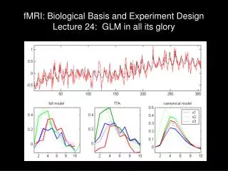
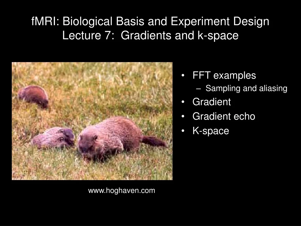
fMRI: Biological Basis and Experiment Design Lecture 7: Gradients and k-space. FFT examples Sampling and aliasing Gradient Gradient echo K-space. www.hoghaven.com. Zooming in k-space is undersampling in real space. Zooming in real space is undersampling in k-space.

E N D
fMRI: Biological Basis and Experiment DesignLecture 7: Gradients and k-space • FFT examples • Sampling and aliasing • Gradient • Gradient echo • K-space www.hoghaven.com
General imaging considerations • K-space resolution (sampling rate) determines field of view (FOV) • Sampling bandwidth, for a fixed read-out gradient, determines FOV • K-space coverage (matrix size) determines resolution • Image "bandwidth per pixel" (different on different axes) determines sensitivity to susceptibility-induced artifacts.
- 0 Gradient echo When a gradient is applied, the spins begin to pick up a phase difference The phase depends on both space and time (and gradient strength) Immediately after excitation, all the spins in a sample are in phase G = 5.1kHz/cm G = 12mT/m B f x x t = 0 s t = 20 s t = 160 s
- 0 Gradient echo B G = -12mT/m Applying a gradient in the opposite direction reverses this process x t = 160 s t = 300 s t = 320 s
- 0 Applying a gradient produces a periodic spin phase pattern GRO Magnitude of signal in RF coil Real part of signal in RF coil Imaginary component of signal in RF coil
- 0 The read-out signal is the 1D FFT of the sample GRO Magnitude of signal in RF coil Real part of signal in RF coil Imaginary component of signal in RF coil
- 0 Applying simultaneous gradients rotates the coordinate system GRO GPE
- 0 Phase encoding allows independent spatial frequency encoding on 2 axes PE Read gradient creates phase evolution while one line of k-space is acquired PE gradient imposes phase pattern on one axis GPE GRO RO Read "refocusing" gradient rewinds phase pattern on another axis
- 0 Phase encoding allows independent spatial frequency encoding on 2 axes PE Read gradient creates phase evolution while one line of k-space is acquired PE gradient imposes phase pattern on one axis GPE GRO RO Read "refocusing" gradient rewinds phase pattern on another axis
- 0 FLASH sequences read one line per excitation Relative phase of spins
Pulse sequence diagram: slow 2D FLASH (64 x 64) Nrep = 64 Flip angle ~ 56 deg. TR ~ 640us RF GSS PE table increments each repetition GPE GRO 64 points DAC
- 0 EPI sequences zig-zag back and forth across k-space
Pulse sequence diagram: EPI (64 x 64 image) Total read-out time ~40 ms Bandwidth (image): 100kHz (dwell time: 10us) Nrep = 32 RF GSS GPE GRO 64 pts 64 pts DAC