Download
1 / 57
570 likes | 584 Vues
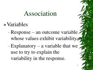
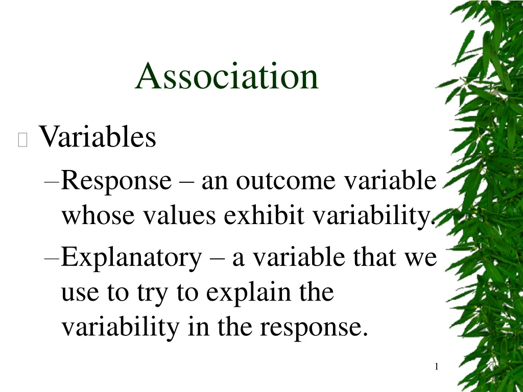
Association. Variables Response – an outcome variable whose values exhibit variability. Explanatory – a variable that we use to try to explain the variability in the response. Association.

E N D
Association • Variables • Response – an outcome variable whose values exhibit variability. • Explanatory – a variable that we use to try to explain the variability in the response.
Association • There is an association between two variables if values of one variable are more likely to occur with certain values of a second variable.
Picturing Association • Two Categorical (Qualitative). • Cross-tabs table, mosaic plot. • Two Numerical (Quantitative). • Scatter diagram.
Categorical Data • Who? • Students in a statistics class at Penn State University. • What? • “With whom is it easiest to make friends?” Opposite sex, same sex, no difference. • Gender. Male, female.
Cross-tabs Table With whom is it easiest to make friends?
Bar Graph With whom is it easiest to make friends?
Percentages With whom is it easiest to make friends?
Interpretation • More that 50% of males say no difference while less than 50% of females say no difference. • Females are about twice as likely as males to say opposite. • Males are about twice as likely as females to say the same.
Scatter Plot • Statistics is about … variation. • Recognize, quantify and try to explain variation. • Variation in two quantitative variables is displayed in a scatter plot.
Scatter Plot • Numerical variable on the vertical axis, y, is the response variable. • Numerical variable on the horizontal axis, x, is the explanatory variable.
Scatter Plot • Example: Body mass (kg) and Bite force (N) for Canidae. • y, Response: Bite force (N) • x, Explanatory: Body mass (kg) • Cases: 28 species of Canidae.
Positive Association • Positive Association • Above average values of Bite force are associated with above average values of Body mass. • Below average values of Bite force are associated with below average values of Body mass.
Scatter Plot • Example: Outside temperature and amount of natural gas used. • Response: Natural gas used (1000 ft3). • Explanatory: Outside temperature (o C). • Cases: 26 days.
Negative Association • Above average values of gas are associated with below average temperatures. • Below average values of gas are associated with above average temperatures.
Association • Positive • As x goes up, y tends to go up. • Negative • As x goes up, y tends to go down.
Correlation • Linear Association • How closely do the points on the scatter plot represent a straight line? • The correlation coefficient gives the direction of and quantifies the strength of the linear association between two quantitative variables.
Correlation • Standardize y • Standardize x
Correlation Coefficient • Body mass and Bite force • r = 0.9807
Correlation Coefficient • There is a very strong positive correlation, linear association, between the body mass and bite force for the various species of Canidae.
JMP • Analyze – Multivariate methods – Multivariate • Y, Columns • Body mass • BF ca (Bite force at the canine)
Correlation Properties • The sign of r indicates the direction of the association. • The value of r is always between –1 and +1. • Correlation has no units. • Correlation is not affected by changes of center or scale.
Algebra Review • The equation of a straight line • y = mx + b • m is the slope – the change in y over the change in x – or rise over run. • b is the y-intercept – the value where the line cuts the y axis.
Review • y = 3x + 2 • x = 0 y = 2 (y-intercept) • x = 3 y = 11 • Change in y (+9) divided by the change in x (+3) gives the slope, 3.
Linear Regression • Example: Body mass (kg) and Bite force (N) for Canidae. • y, Response: Bite force (N) • x, Explanatory: Body mass (kg) • Cases: 28 species of Canidae.
Correlation Coefficient • Body mass and Bite force • r = 0.9807
Correlation Coefficient • There is a strong correlation, linear association, between the body mass and bite force for the various species of Canidae.
Linear Model • The linear model is the equation of a straight line through the data. • A point on the straight line through the data gives a predicted value of y, denoted .
Residual • The difference between the observed value of y and the predicted value of y, , is called the residual. • Residual =
Line of “Best Fit” • There are lots of straight lines that go through the data. • The line of “best fit” is the line for which the sum of squared residuals is the smallest – the least squares line.
Line of “Best Fit” • Some positive and some negative residuals but they sum to zero. • Passes through the point .
Line of “Best Fit” Least squares slope: intercept:
Least Squares Estimates Body mass, x Bite Force, y
Interpretation • Slope – for a 1 kg increase in body mass, the bite force increases, on average, 13.428 N. • Intercept – there is not a reasonable interpretation of the intercept in this context because one wouldn’t see a Canidae with a body mass of 0 kg.
Prediction • Least squares line
Residual • Body mass, x = 25 kg • Bite force, y = 351.5 N • Predicted, = 366.1 N • Residual, = 351.5 – 366.1 = – 14.6 N
Residuals • Residuals help us see if the linear model makes sense. • Plot residuals versus the explanatory variable. • If the plot is a random scatter of points, then the linear model is the best we can do.
Interpretation of the Plot • The residuals are scattered randomly. This indicates that the linear model is an appropriate model for the relationship between body mass and bite force for Canidae.
(r)2 or R2 • The square of the correlation coefficient gives the amount of variation in y, that is accounted for or explained by the linear relationship with x.
Body mass and Bite force • r = 0.9807 • (r)2 = (0.9807)2 = 0.962 or 96.2% • 96.2% of the variation in bite force can be explained by the linear relationship with body mass.