Download
1 / 20
200 likes | 309 Vues
B. A. V BB’ (t). Vg(t). V AA’ (t). L. A’. B’. 16.360 Lecture 4. Last lecture:. Phasor Electromagnetic spectrum Transmission parameters equations . V BB’ (t) = V AA’ (t- t d ) = V AA’ (t-L/c) = V0cos( (t-L/c)) = V0cos( t- 2L/),.

E N D
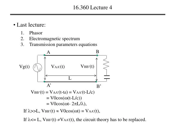
B A VBB’(t) Vg(t) VAA’(t) L A’ B’ 16.360 Lecture 4 • Last lecture: • Phasor • Electromagnetic spectrum • Transmission parameters equations VBB’(t) = VAA’(t-td) = VAA’(t-L/c) = V0cos((t-L/c)) = V0cos(t- 2L/), If >>L, VBB’(t) V0cos(t) = VAA’(t), If <= L, VBB’(t) VAA’(t), the circuit theory has to be replaced.
16.360 Lecture 4 • Today: • Transmission line parameters • Types of transmission lines • Lumped-element model • Transmission line equations • Telegrapher’s equations • Wave equations
B A VBB’(t) Vg(t) VAA’(t) L A’ B’ 16.360 Lecture 4 • Transmission line parameters • time delay VBB’(t) = VAA’(t-td) = VAA’(t-L/vp), • Reflection: the voltage has to be treat as wave, some bounce back • power loss: due to reflection and some other loss mechanism, • Dispersion: in material, Vp could be different for different wavelength
B E 16.360 Lecture 4 • Types of transmission lines • Transverse electromagnetic (TEM) transmission lines B E a) Coaxial line b) Two-wire line c) Parallel-plate line d) Strip line e) Microstrip line
16.360 Lecture 4 • Types of transmission lines • Higher-order transmission lines a) Optical fiber b) Rectangular waveguide c) Coplanar waveguide
16.360 Lecture 4 • Lumped-element Model • Represent transmission lines as parallel-wire configuration A B Vg(t) VBB’(t) VAA’(t) B’ A’ z z z R’z L’z L’z R’z L’z R’z Vg(t) G’z C’z C’z C’z G’z G’z
16.360 Lecture 4 • Transmission line equations • Represent transmission lines as parallel-wire configuration i(z,t) i(z+z,t) L’z R’z V(z,t) V(z+ z,t) G’z C’z V(z,t) = R’z i(z,t) + L’z i(z,t)/ t + V(z+ z,t), (1) i(z,t) = G’z V(z+ z,t) + C’z V(z+ z,t)/t + i(z+z,t), (2)
i(z,t) i(z+z,t) L’z R’z V(z,t) V(z+ z,t) G’z C’z jt jt V(z,t) = Re( V(z) e i (z,t) = Re( i (z) e ), ), 16.360 Lecture 4 • Transmission line equations V(z,t) = R’z i(z,t) + L’z i(z,t)/ t + V(z+ z,t), (1) -V(z+ z,t) + V(z,t) = R’z i(z,t) + L’z i(z,t)/ t - V(z,t)/z = R’ i(z,t) + L’ i(z,t)/ t, (3) Rewrite V(z,t) and i(z,t) as phasors, for sinusoidal V(z,t) and i(z,t):
i(z,t) i(z+z,t) L’z R’z V(z,t) V(z+ z,t) G’z C’z jt e j = Re(i ), - dV(z)/dz = R’ i(z) + jL’ i(z), (4) 16.360 Lecture 4 • Transmission line equations Recall: jt di(t)/dt= Re(d i e )/dt - V(z,t)/z = R’ i(z,t) + L’ i(z,t)/ t, (3)
16.360 Lecture 4 • Transmission line equations • Represent transmission lines as parallel-wire configuration i(z,t) i(z+z,t) L’z R’z V(z,t) V(z+ z,t) G’z C’z V(z,t) = R’z i(z,t) + L’z i(z,t)/ t + V(z+ z,t), (1) i(z,t) = G’z V(z+ z,t) + C’z V(z+ z,t)/t + i(z+z,t), (2)
i(z,t) i(z+z,t) L’z R’z V(z,t) V(z+ z,t) G’z C’z jt jt V(z,t) = Re( V(z) e i (z,t) = Re( i (z) e ), ), 16.360 Lecture 4 • Transmission line equations i(z,t) = G’z V(z+ z,t) + C’z V(z+ z,t)/t + i(z+z,t), (2) - i (z+ z,t) + i (z,t) = G’z V(z + z ,t) + C’z V(z + z,t)/ t - i(z,t)/z = G’ V(z,t) + C’ V(z,t)/ t, (5) Rewrite V(z,t) and i(z,t) as phasors, for sinusoidal V(z,t) and i(z,t):
i(z,t) i(z+z,t) L’z R’z V(z,t) V(z+ z,t) G’z C’z jt e j = Re(V ), - d i(z)/dz = G’ V(z) + jC’ V(z), (7) 16.360 Lecture 4 • Transmission line equations Recall: jt dV(t)/dt= Re(d V e )/dt - i(z,t)/z = G’ V(z,t) + C’ V(z,t)/ t, (6)
i(z,t) i(z+z,t) L’z R’z V(z,t) V(z+ z,t) G’z C’z - d i(z)/dz = G’ V(z) + jC’ V(z), (7) - dV(z)/dz = R’ i(z) + jL’ i(z), (4) - d²V(z)/dz² = R’ di(z)/dz + jL’ di(z)/dz, (8) 16.360 Lecture 4 • Telegrapher’s equation in phasor domain Take d /dz on both sides of eq. (4)
- dV(z)/dz = R’ i(z) + jL’ i(z), (4) - d²V(z)/dz² = R’ di(z)/dz + jL’ di(z)/dz, (8) 16.360 Lecture 4 • Telegrapher’s equation in phasor domain - d i(z)/dz = G’ V(z) + jC’ V(z), (7) substitute (7) to (8) d²V(z)/dz² = (R’ + jL’) (G’+ jC’)V(z), or d²V(z)/dz² - (R’ + jL’) (G’+ jC’)V(z) = 0, (9) d²V(z)/dz² - ²V(z) = 0, (10) ² = (R’ + jL’) (G’+ jC’), (11)
i(z,t) i(z+z,t) L’z R’z V(z,t) V(z+ z,t) G’z C’z - d i(z)/dz = G’ V(z) + jC’ V(z), (7) - dV(z)/dz = R’ i(z) + jL’ i(z), (4) 16.360 Lecture 4 • Telegrapher’s equation in phasor domain Take d /dz on both sides of eq. (7) - d² i(z)/dz² = G’ dV(z)/dz + jC’ dV(z)/dz, (12)
- dV(z)/dz = R’ i(z) + jL’ i(z), (4) 16.360 Lecture 4 • Telegrapher’s equation in phasor domain - d i(z)/dz = G’ V(z) + jC’ V(z), (7) - d² i(z)/dz² = G’ dV(z)/dz + jC’ dV(z)/dz, (12) substitute (4) to (12) d² i(z)/dz² = (R’ + jL’) (G’+ jC’)i(z), or d² i(z)/dz² - (R’ + jL’) (G’+ jC’) i(z) = 0, (9) d² i(z)/dz² - ²i(z) = 0, (13) ² = (R’ + jL’) (G’+ jC’), (11)
= Re (R’ + jL’) (G’+ jC’) , = Im (R’ + jL’) (G’+ jC’) , 16.360 Lecture 4 • Wave equations d²V(z)/dz² - ²V(z) = 0, (10) d² i(z)/dz² - ²i(z) = 0, (13) = + j,
16.360 Lecture 4 • Summary • Transmission line parameters • Types of transmission lines • Lumped-element model • Transmission line equations • Telegrapher’s equations • Wave equations
16.360 Lecture 4 • Next lecture • Wave propagation on a Transmission line • Characteristic impedance • Standing wave and traveling wave • Lossless transmission line • Reflection coefficient