Download
1 / 28
290 likes | 507 Vues
Channel Estimation for IEEE 802.16a OFDM Downlink Transmission. Student: 王依翎 Advisor: Dr. David W. Lin 2006/02/23. Outline. Introduction to IEEE 802.16a Downlink channel estimation methods Simulation. Reference. (1) Ruu-Ching Chen , “IEEE 802.16a TDD OFDMA

E N D
Channel Estimation for IEEE 802.16a OFDM Downlink Transmission Student: 王依翎 Advisor: Dr. David W. Lin 2006/02/23
Outline • Introduction to IEEE 802.16a • Downlink channel estimation methods • Simulation
Reference • (1) Ruu-Ching Chen, “IEEE 802.16a TDD OFDMA Downlink Pilot-Symbol-Aided Channel Estimation: Techniques and DSP Software Implementation ,“ M.S. thesis, Department of Electronics Engineering, National Chiao Tung University, Hsinchu ,Taiwan, R.O.C., June 2005. • (2) IEEE Std 802.16a-2003, IEEE Standard for Local and Metropolitan Area Networks - Part 16: Air Interface for Fixed Broadband Wireless Access Systems – Amendment 2: Medium Access Control Modifications and Additional Physical Layer Specifications for 2-11GHz. New York: IEEE, April 1, 2003.
Outline • Introduction to IEEE 802.16a • Downlink channel estimation methods • Simulation
Primitive Parameters • Primitive parameters characterize the OFDMA symbol: (1) BW : the nominal channel bandwidth, it equals 10 MHz in the system . (2) Fs/BW : the ratio of “sampling frequency" to the nominal channel bandwidth. It is set to 8/7. (3)Tg/Tb : the ratio of CP time to “useful" time. We use 1/8 in the system. (4) NFFT: the number of points in the FFT. The OFDMA PHY defines this value to be 2048.
Derived Parameters • The following parameters are defined in terms of the primitive parameters. (1)Fs = (Fs/BW)‧BW = sampling frequency. The value equals 10X8/7 = 11.42 MHz. (2)Δf = Fs/NFFT = carrier spacing = 5.57617 KHz. (3)Tb = 1/Δf = useful time = 179.33 μs. (4)Tg = (Tg/Tb)‧Tb = CP time = 22.4 μs. (5)Ts = Tb + Tg = OFDM symbol time = 201.9μs. (6)1/Fs = sample time = 87.5657 ns.
Pilot Allocation varLocPilotk= 3L + 12Pk ,Pk={0,1,2,……,141}
Data Carrier Allocation • The exact partitioning into subchannels is according to the following equation called a permutation formula:
Pilot Modulation • The polynomial • for the PRBS • generator is
Outline • Introduction to IEEE 802.16a • Downlink channel estimation methods • Simulation
DL Channel Estimation Methods • Our interpolation schemes work in both frequency and the time domains. (1)Linear and second-order interpolation are applied in the frequency domain (2)2-D interpolation and LMS (least mean square adaptation) optimize their performance in the time domain.
Least-Square (LS) Estimator • An LS estimator minimizes the squared error : where Y : the received signal X : a priori known pilots • Channel matrix considering pilot carriers only: →
Least-Square (LS) Estimator (cont.) • The estimate of pilot signals, based on one observed OFDM symbol, is given by where N(m) is the complex white Gaussian noise on subcarrier m • The LS estimate of Hp based on one OFDM symbol only is susceptible to Gaussian noise, and thus an estimator better than the LS estimator is preferable.
Linear Minimum Mean Squared Error (LMMSE) Estimator • The mathematical representation for the LMMSE estimator of pilot signals is where the covariance matrices are defined by
Linear Interpolation • Mathematical expression: where Hp(k); k = 0,1,…,Np, are the channel frequency responses at pilot subcarriers, L is the distance between the two given data,the pilot sub-carriers spacing, and 0 ≦ l < L.
Second-Order Interpolation • Also called Gaussian second order estimation. • The interpolation is obtained using three successive pilot subcarriers signal as follows : where
Time Domain Improvement Methods • We can only use 166 pilots in one symbol to interpolate the channel in the frequency domain. • It is not sufficient because the pilot spacings are too wide in our system. • Since the channel does not change abruptly over time, we propose two methods to improve the performance. (1) Two-Dimensional Interpolation (2) Least Mean Square (LMS) Adaptation
Two-Dimensional Interpolation • Index of a variable location pilot : • The maximum number of pilot locations that we can use is : • Since the equivalent number of pilots becomes 568/166 = 3.421 times that of the original case, better estimation is expected.
Two-Dimensional Interpolation (cont.) • One possible way of interpolation (extrapolation) is where , n = 0, 1, … , 7, are the channel frequency responses at pilot carriers in the nth previous symbol. • When dealing with fading channels, we consider replacing the formula above with (formula 1) (formula 2)
Least Mean Square (LMS) Adaptation • The LMS algorithm is the most widely used adaptive filtering algorithm in practice for its simplicity.
Outline • Introduction to IEEE 802.16a • Downlink channel estimation methods • Simulation
Comparison Between Formula 1 and Formula 2 Using Linear Interpolation • SER : (symbol error rate)
Comparison Between Formula 1 and Formula 2 Using Linear Interpolation (cont.) • MSE of : (mean square error)
Comparison Between Formula 1 and Formula 2 Using 2nd-Order Interpolation • SER
Comparison Between Formula 1 and Formula 2 Using 2nd-Order Interpolation (cont.) • MSE of :