Download
1 / 12
120 likes | 245 Vues
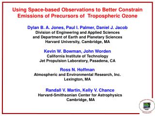
Assessment of the Potential of Observations from TES to Constrain Emissions of Carbon Monoxide. Dylan B. A. Jones, Paul I. Palmer, Daniel J. Jacob Division of Engineering and Applied Sciences, and Department of Earth and Planetary Sciences, Harvard University, Cambridge, MA.

E N D
Assessment of the Potential of Observations from TES to Constrain Emissions of Carbon Monoxide Dylan B. A. Jones, Paul I. Palmer, Daniel J. Jacob Division of Engineering and Applied Sciences, and Department of Earth and Planetary Sciences, Harvard University, Cambridge, MA Kevin W. Bowman, John Worden California Institute of Technology,Jet Propulsion Laboratory, Pasadena, CA Ross N. Hoffman Atmospheric and Environmental Research, Inc. Lexington, MA September 19, 2002
OBJECTIVE: Determine whether nadir observations of CO from TES (Tropospheric Emission Spectrometer) will have enough information to reduce uncertainties in our estimates of regional sources of CO APPROACH: Use the GEOS-CHEM 3-D model together with calculated averaging kernels for TES to simulate TES nadir retrievals of CO Use an optimal estimation inverse method to infer the sources of CO from the TES retrievals
Source Distribution EUFF NAFF ASFF ASBB AFBB CHEM SABB RWFF RWBB • FF = Fossil Fuel + Biofuel • All sources include contributions from oxidation of VOCs • OH is specified • Use a “tagged CO” method to estimate contribution from each source • Use inverse method to solve for annually-averaged emissions “True” Emissions (Tg/yr) NAFF: 121.3 SABB: 96.5 EUFF: 131.1 RWBB: 98.0 ASFF: 258.3 RWFF: 149.8 ASBB: 96.0 CHEM: 1125.0 AFBB: 193.9 Total = 2270 Tg/yr
P > 250 mb Simulating the Data • Sample the synthetic atmosphere along the orbit of TES • The retrieved profile is: yret = ya + A(F(xt) – ya) ya = a priori profile xt = true emissions yt = F(xt) F(x) = GEOS-CHEM A = averaging kernels yret ya
Methodology Use a sequential non-linear least squares solver to minimize a maximum a posteriori cost function x = CO sources (state vector) xa = a priori estimate of the sources yret = retrieved profile F(x) = forward model A = Averaging kernels Sx = error covariance of sources Sy = error covariance of observations = instrument error (Si) + model error (Sm)+ representativeness error (Sr)
The Forward Model We apply the same ya and A used for the retrieved profileto GEOS-CHEM (forward model) } The retrieved profile andthe forward model mustbe consistent G = gain matrix associated with A ei = r.m.s of instrument noiseSi = G<(ein)(ein)T>GT n = Gaussian white noise with unity variance Gein = instrument noise e = model noise based on error patterns of (Sm + Sr) lj and ej are j th eigenvalue and eigenvectorof (Sm + Sr) (Sr)jj = 5%, based on TRACE-P aircraft data
Constructing the Covariance Matrix for the Model Error • Compare model with observations of CO from TRACE-P and estimate the relative error • Assume mean bias in relative error is due to emission errors • Remove mean bias and assume the residual relative error (RRE) is due to transport • Small RRE in background air (low CO) • Large RRE if model incorrectly predicts plume : (COmod small and COobs large or vice versa) 6 – 8 km |log(COmod/COobs)| Fit the absolute values of log(COmod/COobs) vs. Max. (COmod or COobs) CO (ppb)
Model Error Model Level 16 (8 km) March 15 2001 0 GMT Model Level 8 (1.5 km)
Assumptions • Assume that sources are uncorrelated with uncertainty(Sx)jj = 50% (for the chemistry source we assume 25%) • Assume that the transport errors are spatially uncorrelated • Cloud free conditions • We use the same averaging kernels for all profile retrievals • We consider data only between the equator and 60ºN • We use only 5 days of simulated data, March10-15th, 2001
a priori a posteriori true Inversion Results Model successfully retrieves the true emissions for all sources caveat: perfect Gaussian error statistics with zero bias
How well do we constrain the sources with only upper tropospheric (P < 500 hPa) observations? Good constraint, but errors are larger ( ~ x 2, for most sources) lower tropospheric retrievals provide useful additional information
Conclusions • TES retrievals of CO have the potential to constrain regional sources of CO, but proper error characterization will be crucial; real data will not have unbiased Gaussian error statistics which will reduce the information we can extract • Upper tropospheric retrievals alone may provide considerable information to constrain the sources • Since most of the CO information is in the lower troposphere, TES retrievals below 500 hPa will be useful in constraining the sources, despite the instrument’s reduced sensitivity in the lower troposphere • Future work • Inversion analysis with CO retrievals from SCIAMACHY