Download
1 / 14
150 likes | 167 Vues
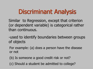
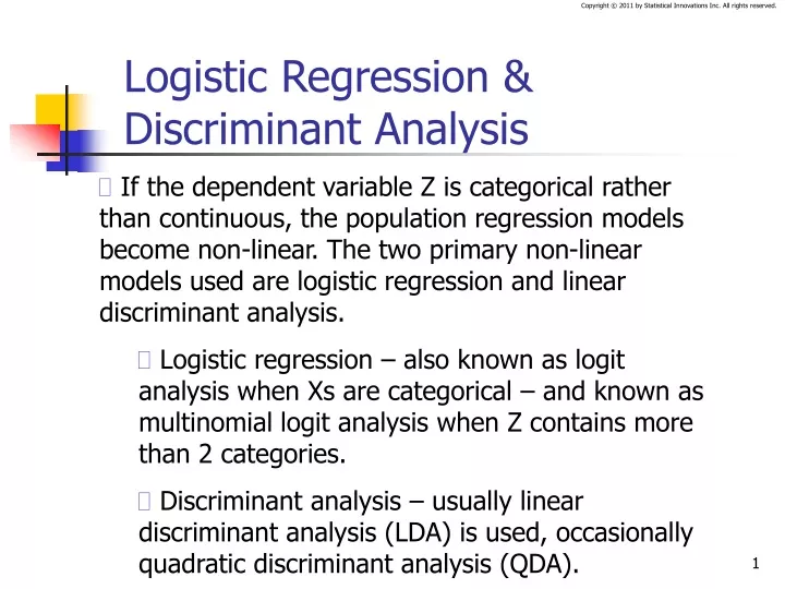
Logistic Regression & Discriminant Analysis. If the dependent variable Z is categorical rather than continuous, the population regression models become non-linear. The two primary non-linear models used are logistic regression and linear discriminant analysis.

E N D
Logistic Regression & Discriminant Analysis • If the dependent variable Z is categorical rather than continuous, the population regression models become non-linear. The two primary non-linear models used are logistic regression and linear discriminant analysis. • Logistic regression – also known as logit analysis when Xs are categorical – and known as multinomial logit analysis when Z contains more than 2 categories. • Discriminant analysis – usually linear discriminant analysis (LDA) is used, occasionally quadratic discriminant analysis (QDA).
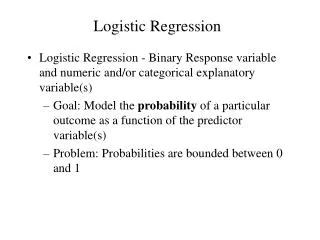
Dichotomous Dependent Variable • Here we provide some basics for logistic regression and discriminant analysis for dependent variable Z dichotomous, say Z = 1,0. The conditional expectation of Z given X then simplifies to the probability that Z=1: • E(Z|X) = prob(Z=1|X)*1 + prob(Z=0|X)*0 = prob(Z=1|X) • Since probabilities are bounded, the linear regression model Prob(Z=1|X)=XB is no longer appropriate.
PROB 1.0 XB = (probability) 0 Note: Probabilities can be less than 0 or greater than 1 as estimated by OLS or GLS.
Logit or Log-Odds Units In dealing with dichotomous dependent variables it is useful to work in units of odds (and log-odds) rather than probabilities in order to express the non-linear model in a linear form. Some definitions: Some useful equations for logistic distribution: PROB(Z=1|X) = eXB / (1+ eXB) PROB(Z=0|X) = 1/ (1+ eXB) Thus,
Logistic Regression PROB(Z=1|X) = eXB / (1+ eXB) 1.0 Logistic regression is a non-linear probability model but linear (as a logit model) when re-expressed in logit (log-odds) units. 0.5 XB = (logit) 0 Prob = .5 translates into Odds = 1.0 or Logit = 0
Correct Classification Rates: Classification Tables Measure Accuracy of Prediction Given the predicted logit score Li for respondent i from a given model, predict (classify) that respondent as follows: Predict Z=1 if Li > c, Predict Z=0 if Li≤ c Where cut-point c = 0 usually (corresponding to predicted prob = .5) Simulated data example: Models estimated on training data (N1 = N2 = 25), and applied to Validation data (N1 = N2 = 2,500). Sensitivity = 92.2% P(Li > c|ZPC1 = 1) Specificity = 91.8% P(Li≤ c|ZPC1 = 0) Accuracy = (2295 + 2305)/5000 = 92% AUC = .978
Area Under Curve (AUC) Statistic ROC curve plots the sensitivity and specificity for every possible cut-point. Irrelevant model score yields diagonal ROC (green line), with AUC = .5. AUC represents the probability that a randomly selected case from group 1 will have a higher model score than a randomly selected case from group 2. Above, AUC = .978 for blue ROC curve. Cut-point = 0 Sensitivity = 92.2% Specificity = 91.8%
Linear Discriminant Analysis • Alternative approach to estimate regression coefficients in logistic regression model • Appropriate when Xs are treated as random and continuous.
Assumptions Made in Linear Discriminant Analysis (LDA) • The vector of predictor variables X follows a multivariate normal distribution within each group Z=1 & Z=0 • The variance-covariance matrix is identical within each Z group • Note: If is not identical within each group, get quadratic equation (QDA)
Comparison of LDA vs. Logit Analysis • Under LDA assumptions it follows that: • the discriminant function is linear in X • predicted probability of Z=1 follows logistic distribution • coefficient estimates more efficient than logistic regression approach. • However, if X contains some dichotomous (or polytomous) variables, the LDA may result in serious biases, since • the discriminant function will in general not be linear but will include interaction terms.
Logistic Regression Alternative • Estimate the probabilities of group membership directly (bypass the discriminant function) • No assumption of normality • Recommended by some statisticians over discriminant analysis even when X is multivariate normal • If all predictors are categorical, log-linear modeling software can be used (“logit analysis”)
Numerical problems • Collinearity and near-collinearity can occur in logistic regression and LDA just as in ordinary regression. • Logistic regression also has another problem called (perfect) separation.
Data Illustrating Perfect Separation X treated as continuous X values below 6 all indicate Y=1 X values at or above 6 all indicate Y=1
Fitted Model Estimates for B are not unique. ML estimate for B is –infinity. ‘Failure to converge’ warning from SPSS Logistic Regression. Latent GOLD output produces a warning message telling you that the solution is not identifiable (i.e., not unique): “1-Class Ordinal Regression Model Estimation Warnings! See Iteration Detail”