Download
1 / 31
310 likes | 316 Vues
This text discusses the measurements and parameterization of turbulent fluxes of heat, moisture, and momentum in the atmosphere. It explains the eddy correlation method and the instrumentation used for direct measurements. It also explores the relationship between stress and vertical wind distribution and the role of friction velocity and roughness length in determining wind speed. The text highlights the importance of accurately measuring these parameters for understanding surface turbulent fluxes.

E N D
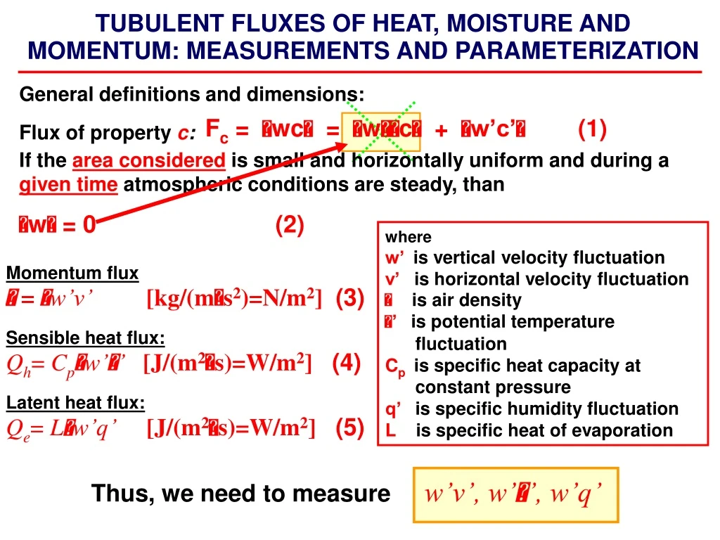
Fc = wc= wc+ w’c’(1) TUBULENT FLUXES OF HEAT, MOISTURE AND MOMENTUM: MEASUREMENTS AND PARAMETERIZATION General definitions and dimensions: Flux of property c: If the area considered is small and horizontally uniform and during a given time atmospheric conditions are steady, than w = 0 (2) where w’ is vertical velocity fluctuation v’ is horizontal velocity fluctuation is air density ’ is potential temperature fluctuation Cp is specific heat capacity at constant pressure q’ is specific humidity fluctuation L is specific heat of evaporation Momentum flux = w’v’ [kg/(ms2)=N/m2] (3) Sensible heat flux: Qh= Cpw’’ [J/(m2s)=W/m2] (4) Latent heat flux: Qe= Lw’q’ [J/(m2s)=W/m2] (5) Thus, we need to measure w’v’, w’’, w’q’
The eddy correlation method • Statistical meaning of fluxes: • w’v’, w’’, w’q’ can be considered as the • second mixed moments, i.e. • co-variances of variables • Requirements for the direct measurements • Covariances should be measured, and • not the variances • Time resolution should be high (10-20 Hz) • The record should be relatively long • (more than 20 min) • Instrumentation: • Sonic anemometer • Fast-response thermometer • Fast-response infrared hydrometer ship Stationary platform • Problems: • Technically difficult • Expensive
Sonic anemometer is based on the estimation of speed of sound V = [(t1-t2)C2] / 2d We need to measure variances of wind velocity in 3 directions Description of a typical eddy correlation package: The 3-D sonic anemometer uses three pairs of orthogonally oriented, ultrasonic transmit/receive transducers to measure the transit time of sound signals traveling between the transducer pairs. The wind speed along each transducer axis is determined from the difference in transit times. The sonic temperature is computed from the speed of sound which is determined from the average transit time along the vertical axis. A pair of measurements are made along each axis normally 100 times per second. 10 measurements are averaged to produce 10 wind measurements along each axis and 10 temperatures each second. The infrared hygrometer measures the water vapor density by detecting the absorption of infrared radiation by water vapor in the light path. Two infrared wavelength bands are used, one centered on a band strongly absorbed by water vapor, and one centered on a band (the reference band) which is not absorbed. By normalizing the absorption band by the reference band, instrument drifts caused by light source and photo-detector changes are eliminated. Measurements are made 40 times per second. 4 measurements are averaged to produce 10 water vapor density measurements each second.
Parameterization of surface turbulent fluxes massively measured SST, Ta, q, V, SLP parameterization w’v’, w’’, w’q’ What should be a combination of massively measured parameters to be compared with direct flux measurements? From K-theory the relationship between stress and vertical distribution of wind under stationary conditions: Kmis eddy diffusivity ~ [m2s-1] ~ [UL] u/zis the velocity gradient ~ [s-1] ~ [U/L] Km(u/z) ~ [U2] What is this velocity? This is the velocity related to the mean speed of turbulent eddies u*. Now for the stress: i.e. the eddy velocities in neutral conditions are independent on the height. (10)
/u* u ln z Velocity u* is called friction velocity and serves as indicator of velocity scale in the exchange theory. It is proportional to root-mean square vertical velocity: u* ~ w We need to know also the size of the largest eddies. It is related to the height, because the upper limit of eddy is determined by the distance from the sea surface. Thus, for Km: Where is the von Karman constant of proportionality (0.4) Km:= u*z (11) non-dimensional wind shear (12) Measurements of mean velocity at several levels, plotted on a log-scale give a straight live with a slope of /u*
Integration of (12) gives equation for the vertical distribution of mean velocity: z0 is the integration constant. It represents the height, on which the mean wind speed calculated by (13) goes to zero. This is the so-called roughness length. (13) Land data: We can calculate friction velocity and wind speed at any level step by step Von Karman constant
Dimensional analysis under light wind speed when the ocean surface is smooth shows that: z0 ~ /u*however, no observational evidence has been found for that, except for Roll (1961). Henry Charnock (1955) assumed that roughness lenght depends on surface stress and gravity, and derived experimental formula: Sea surface: • the shape of the surface and the roughness lengths vary with • wind speed; • marine roughness length may depend on the characteristics of • short capillary waves, but does not depend on longer waves (sea); • wind sea is not what the roughness length is about!!! • marine roughness elements are not stationary, they move • together with significant waves. z0 = 0.0123u*2 / g(14) where 0.0123 is the Charnock «constant», which varies in different studies from 0.011 to 0.018.
On aerodynamically smooth surfaces the stress is exerted by viscosity and within the laminar sublayer the stress is proportional to wind speed z0 ~ /u* On rough surfaces, the effects of viscosity are negligible and the transfer of stress to the surface is done by the pressure differences between the upwind and downwind sides of the obstacles z0 = 0.0123u*2 / g under neutral conditions: neutral drag coefficient: Stress: (15)
Passive mean properties under neutral conditions (,q) For the potential temperature and humidity with the use of K-theory: (16) Eddy diffusivity for humidity Eddy diffusivity for temperature We introduce now (with the analogy to u*) two new scales: q* and * (17) For non-dimensional temperature and humidity gradients: (18) Ratio of exchange coefficients for passive property and momentum is a fundamental question of boundary layer turbulence. In general, it depends on stability, but for the neutral conditions can be taken as constant.
lnz /q* q Measurements of mean velocity at several levels, plotted on a log-scale give a straight live with a slope of /q* Unlike the momentum, the mean values of θ, q do not approach zero at the surface, but come to the values which depend on the processes at the surface. Let’s define them as θa, qaand integrate (18): Integration constants zaθ and zaqare the heights at which <θ> and <q> are equal to the surface values θa and qa. Although these are analogues of the roughness length, the mechanisms producing zaθ and zaq are completely different from those for zaq.
under neutral conditions: Bulk formulas for the transfer of sensible heat and moisture (still under the neutral conditions) neutral coefficients for heat and moisture transfer:
Ct=? Now, if theconditions are neutral, we can: 1. Measure the mean variables and derive the already known product u(SST-) 2. Measure the flux directly using eddy correlation method • 3. Try to statistically compare these two (SST-Ta) V w’’ But!!!! what to do when the conditions are not neutral??? In this case we have to account for the modification of profiles of wind and passive properties due to surface layer instability.
We have to consider the balance of turbulent kinetic energy Turbulent kinetic energy per unit mass: (21) Reynolds averaging of TKE: (22) The energy of mean motion The eddy energy Equation of TKE transformation can be derived theoretically: see, e.g. Blackadar, A. “Turbulence an diffusion in the atmosphere”.We will consider it as a generally assumed conservation equation of energy.
Conservation of the total kinetic energy: Transformation to and from mechanical energy (23) Work done by stress at boundary Transformation through the potential energy Transformation to and from internal energy External sources
Steps skipped (Blackadar 1997, Appendix A): 1) Reynolds averaging of the total kinetic energy of conservation: (24) 2) Multiplication of the Reynolds averaged Navier-Stockes equation term-by-term by ui and summing over i: (25) 3) Subtraction (25) from (24) term by term: (26)
(27) Production of TKE by buoyancy (+/-) (reversible) TKE transform into internal energy (+) irreversible Mechanical production of TKE (normally positive) External sources (with either sign)
The mechanical production rate (from K-theory): (28) The buoyant production rate (in the dry atmosphere): (29) dry adiabatic lapse rate Ri– gradient Richardson number The flux Richardson number: (30) Ri defines the stability: Richardson argued that when Rf>1 (stable), turbulence does not occur.Later observations and theory have shown that Rc (critical Ri) is about 0.25.
Height on which the two rates of TKE production are equal gives the length scale, known as Monin-Obukhov length: (31) • independent on height • has the same sign as the Richardson number, defining the stability • falls to infinity under neutral conditions Now we can derive a non-dimensional height: z L , (32) which gives the length scale and implies similarity of wind profiles (Monin-Obukhov 1954): Universal function to be estimated (33)
ln z unstable neutral stable U Estimation of (): (34) 1. KEYPS – equation: Sellers Panofsky Yamamoto Ellison Kazansky Solution exists but it is not convenient to use 2. Bussinger et al. (1971) from the experiments in Kansas: 3. Dyer (1974): 4. Large and Pond (1981):
General formulation: (35) Similarity functions for temperature and humidity: Now we can finally derive the bulk formulae!!!
Since we need to estimate flux at a given height z, the equations: should be integrated from the surface to this height, that gives the values of mean variables at height z: Stability correction functions, which are the integrals of non- dimensional profiles (Paulson 1970): (36) (37)
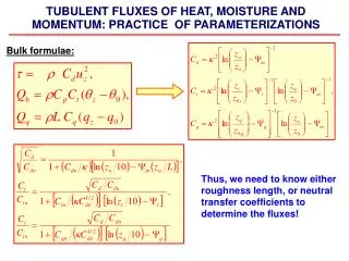
Bulk formulae: (38) Problem of transfer coefficients: neutral coefficients at a given reference height (h=10m): Thus, we need to know either the roughness length, or the neutral transfer coefficients to determine the fluxes!
Inertial dissipation method: TKE – equation: XE for the steady horizontally homogeneous flow: Vertical divergence of turbulent transport Vertical divergence of pressure transport Scaling parameter: z u*3
McBean and Elliott (1975): is independent on L Large and Pond (1981): Very important: this does not mean that bothU , Pare small (a very mistake of many), simply they balance each other. We do not neglect termsXUandXP, but we neglect the sum of these two! Now we can assume: B + P = (39) (40) or Surprise!!!!: if we know , we can find u*!!!!!!!!!!!
How to know ? Attribute of turbulence No.5 from the last lecture: Turbulence is dissipative by nature Molecular destruction of turbulent motions is largest for the smallest size eddies. Thus, if we have only “very small eddies”, they will be destructed by molecular processes and turbulence will decay. But from where “the smallest eddies” come from? Only from the lager scale eddies Thus, there should be a dissipation which allows larger scale eddies to become smaller. And the more intense small scale turbulence is, the greater rate of dissipation occurs. As a consequence, dissipation, as well as the other terms in the TKE equation should depend on the size of eddies. This allows us to consider the TKE equation in a spectral form, where the contributions of terms will depend on the wave length or the eddy size
TKE large eddies small eddies Traditional TKE equation, assuming that the vertical divergence of turbulent transport and pressure transport are neglected and the flow is steady: Let’s assume that we observed that this works for a particular environment during a given time: Let’s assume that we are able to estimate all terms for the eddies of different sizes. Now, let’s plot TKE vs eddy size (wave number) ? Is it also valid for the particular range of the eddy sizes?
Spectral representation of TKE equation (Batchelor 1953, Stull 1988): Viscous dissipation of the k-th component of TKE Mechanical production associated with the k-th component of <w’u’> The local time tendency of the k-th component of TKE Buoyant production associated with the k-th component of <w’’> Convergence of TKE transport across the spectrum
S Generation of TKE Viscosity Small eddies Large eddies Mid-size eddies feel neither the effect of viscosity nor the generation. How do they get their energy? How do they loss it? The cascade rate of energy down the spectrum must balance the dissipation • rate at the smallest eddies sizes. Here eddies get the energy inertially from the larger size eddies and loss it in the same way to smaller size eddies! Kolmogorov (1941), Obukhov (1941): K is the Kolmogorov constant (0.5510%)
Spatial structure of turbulence: frozen turbulence (Taylor 1938): If the mean wind U is directed in x-direction, spatial statistics of U can be considered, assuming that the U(x) is frozen in time, i.e. these statistics move along the x-axis with the mean speed U. k = f / U, f = /2 links time and space for turbulent motion Now we can re-write the Kolmogorov’s hypothesis: (41) But now we can measure the time series of, e.g. wind speed at high frequency and derive the friction velocity from (40), (41): (42)
For the fluxes of passive scalars you need to determine the spectral level of fluctuations in the inertial sub-range and solve the budget equation for this scalar: Spectral similarity Kolmogorov’s constant pertaining to q dissipation function for q
Summary of inertial dissipation method: So, you do not need to measure <w’x’> anymore, you now need only: • Make fast response measurements of velocity to get the time series • Calculate the spectrum of the time series • Plot the spectra on log-log graph • Find inertial subrange, i.e. the portion of the spectrum that exhibits a –5/3 slope • Fit a strait line to this part of your graph • Pick any point on this line and determine the values of S and k • Compute mean wind speed U during your measurements • Solve the equation for : 9. Find wind sress: Find sensible and latent fluxes: