Download
1 / 53
530 likes | 772 Vues
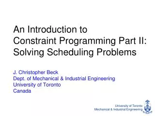
An Introduction to Constraint Programming Part II: Solving Scheduling Problems. J. Christopher Beck Dept. of Mechanical & Industrial Engineering University of Toronto Canada. Where We Left Off …. CP has been mostly developed to solve combinatorial feasibility and optimization problems

E N D
An Introduction toConstraint Programming Part II:Solving Scheduling Problems J. Christopher BeckDept. of Mechanical & Industrial EngineeringUniversity of TorontoCanada
Where We Left Off … • CP has been mostly developed to solve combinatorial feasibility and optimization problems • General solution approach: tree search with inference at each node • no generic relaxation • Key concept: global constraint propagation
Global Constraints • A constraint over an arbitrary number of variables that embodies a frequently encountered sub-problem • all-different(v1, …, vk), global cardinality • disjunctive/cumulative resource • grammar • … • [still some arguments about this within CP] Global Constraint Catalog www.emn.fr/z-info/sdemasse/gccat/index.html
Global Constraints • A global constraint representsa commonly occurring problemsubstructure • The focus of modeling and solving techniques • models are conjunctions of global constraints • solving is typically tree search with domain consistency enforced at every node
Differences with MIP • Richer, extensible language • Focus on global constraints • Traditionally no explicit use of lower bounds • no optimization function • constraint satisfaction problems • less focus on relaxations • less true now: LBs “inside” global constraints
When to Choose CP • <Handwaving mode on> • Finding a feasible solution is hard • intricate set of complicated constraints • No tight relaxations • Existing global constraints model parts of your problem • Strong back-propagation
Operation/Task/ Activity Job Precedence Constraint Job Shop Scheduling
makespan Job Shop Scheduling
Notation estj ectj lstj lctj pj pj – processing time of activity j (aka duration) estj – earliest start time of activity j lstj – latest start time of activity j ectj – earliest completion time of activity j lctj – latest completion time of activity j
Notation [estj lstj] [ectj lctj] pj Domain of start times (represented by an interval)
20 15 10 15 0 Temporal Propagation(Arc Consistency - AC) The same as CPM [0 40] [20 60] [35 75] [45 85] 20 15 10 15 0 100 20 [20 40] [40 60] [55 75] [65 85] 100
20 35 80 Simplified Edge-Finding (aka Constraint-Based Analysis (CBA)) • What can you infer here? 15 50 90 Operations on the same unary capacity resource
25 20 10 15 15 0 10 80 100 est(S) S lct(S) Edge-Finding Exclusion
70 100 25 20 10 15 15 0 75 10 100 est(S) S lct(S) Edge-Finding Exclusion
On the sameunary-capacity resource estA est(S) + dur(S) lftA lft(S) - dur(S) (lft(S) - est(S) < durA + dur(S)) (lft(S) - estA < durA + dur(S)) (lft(S) - est(S) < durA + dur(S)) (lftA - est(S) < durA + dur(S)) Exclusion Rules For all non-empty subsets, S, and activities AS:
Algorithm [Vilim et al 05] • With a clever data structure (Θ-Λ-trees) a set of activities can be updated in O(n log n) time • An easier-to-understand algorithm can do it in O(n2) [Nuijten 1994]
CP vs. MIP for JSP Mean relative error vs. best known solution
Schedule Schedule Schedule Resource Allocation & Scheduling Assign jobs [Hooker 2005] Constraints, 10, 385-401, 2005.
CP Model minimize cost of assignment all jobs assign to 1 resource global resource constraint bounds on start time var. [Heinz & Beck 2012] CPAIOR 2011.
MIP Time-indexed Model resource capacity at each time point
Logic-Based Benders Decomp. Global Model Master Problem Cut Cut Solution Solution Subproblem 1 Subproblem n . . . [Hooker & Ottosson 2003] Mathematical Programming,96, 33-60, 2003.
Assignment Cuts The Approach Assign jobs • Assign jobs to resources subject to sub-problem relaxation and Benders cuts • Schedule independently • Send Benders cuts back to master • Repeat
LBBD Model SP relaxation MP Benders cuts global resource constraint SP [Hooker 2005] Constraints, 10, 385-401, 2005.
Results Number problems (out of 195) for which each method found: [Heinz & Beck 2012] CPAIOR 2012.
Better LBBD tighter SP relaxation [Hooker 2007] Operations Research 55 2013.
New MIP Model redundant variables use tighter SP relaxation from LBBS as a redundant resource capacity constraint [Heinz, Ku, & Beck 2013] CPAIOR 2013.
Results [Heinz, Ku, & Beck 2013] CPAIOR 2013.
Conclusions from Experiments • CP is worst? • well, it finds very high quality solutions is a very short time • MIP is still a very strong technology even for scheduling problems • Hybrids! • CP is a key part of LBBD • I didn’t show you the main point of the paper …
Full Results CIP = constraint integer programming [Heinz, Ku, & Beck 2013] CPAIOR 2013.
OR CP/OR Integration 1 • OR inside • For years CP has been using OR algorithms “inside” global constraints • edge-finding, all-diff, etc. Cost-based pruning in TSPTW
CP/OR Integration 2 • Cooperating solvers, solving the same problem • Model the problem in CP, model the problem in MP, solvers communicate through the variables • MP is “master” and CP suppliesnew implied constraints • CP is “master” and MP supplies lowerbounds, relaxed optimal solutions, etc. • Higher level control: dynamic “master-slave” relationship ETSP
CP/OR Integration 3 • Decomposition • Overall problem is divided between CP and MP solvers • Benders decomposition (MP master, CP slave) • Column generation Column generation Benders decomposition
CP/OR Integration 4 • Deep integration • incorporation global constraint inference into a MIP search • Constraint Integer Programming: SCIP • SIMPL
MIE1619:Constraint Programming &Local Search J. Christopher BeckDept. of Mechanical & Industrial EngineeringUniversity of TorontoCanada
Advanced Grad Course • Course is for “doctoral stream” students • This will be a challenging course • 1-2 papers to read per week • 10-15 hours/week outside lectures • I expect a high-level of performance both in class participation and in the project • Expected level: publishable!
Goals • Apply Constraint Programming (CP) and/or Local Search (LS) to your research interests • Teach “grad school” skills • Literature research, algorithmic research, writing research papers, writing peer reviews, giving presentations, being an active member of the research community
Research Paper Goal • Apply CP and/or LS to your research topic • I have some ideas for people who are stuck • Publish! • The goal (but not a requirement) • The paper you hand in for this course should be publishable • And usable as part of your thesis
Lecture Goal • Doing the readings is essential • You are expected to participate each week • I will ask people to explain particular points • Starting in Week 3, you will begin preparing questions based on the readings
Outline • Intro: 1 week • CP: 3 weeks • LS: 2 weeks • Writing Peer Reviews: 0.5 weeks • OR/CP/LS Hybrids: 4.5 weeks • Project Presentations: 1 or 2 weeks
Search: Texture Measurements • Algorithms for the analysis of the constraint graph representation of a search state • Heuristic search idea: • Use texture measurement to reveal problem structure • Formulate heuristic commitment based on the structure
The SumHeight Heuristic Find the resource, R*, and time point, t*, with highest competition Find the 2 activities not sequenced with each other with the highest individual demand for R* at t* Heuristically, post a sequencing constraint between them
The SumHeight Texture: Individual Demand individual demand for R2 time A1 est ect lst lct
aggregate demand for R2 time The SumHeight Texture: Aggregate Demand Dynamic Focus of Attention R2 R2 R2
Search • At each node (after propagation) • recalculate texture measurements • identify peaks • identify activity pair, A, B • branch on (A B) OR (B A) • See [Beck 1999] for more than you want to know about this