Download
1 / 21
220 likes | 573 Vues
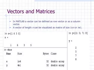
Vectors and Matrices. Lecture Basic vector & matrix concepts Creating arrays and matrices Accessing matrix components Manipulating matrices Matrix functions Solving simultaneous equations. Learning Objectives Understand the nature of matrices

E N D
Vectors and Matrices Lecture • Basic vector & matrix concepts • Creating arrays and matrices • Accessing matrix components • Manipulating matrices • Matrix functions • Solving simultaneous equations Learning Objectives Understand the nature of matrices Understand how to manipulate matrices in Matlab AE6382 Design Computing
Using Matlab with Arrays and Matrices • Matlab’s origins are in the early efforts to develop fast and efficient programs for handling linear equations… • Operations with arrays, vectors and matrices are needed • Only the most computationally efficient routines are used • Matlab is very “C-like” but adds a number of operators and extends its syntax to handle a range of array, vector and matrix operations • Matlab’s fundamental data structure is the array and vectors and matrices follow easily • BUT… to see some of the power of Matlab for engineering applications, we’ll have to dig a bit more deeply into some of the underlying math (no, this is not going to turn into a math class, but it’s often hard to avoid math in engineering) AE6382 Design Computing
Basic Concepts Scalars: magnitude only x, mass, color, 13.451 Vectors: magnitude AND direction Arrays: can be 2D or higher dimension AE6382 Design Computing
Matlab Can Handle This… Scalars: >> whos Name Size Bytes Class a 1x1 8 double array density 1x1 8 double array mass 1x1 8 double array resistance 1x1 8 double array s 1x1 8 double array stress 1x1 8 double array Vectors: >> force=[12.3, 5.67] force = 12.3000 5.6700 >> hvec=[1, 5, -3, 4, 0] hvec = 1 5 -3 4 0 Arrays: >> coef=[1, 2; -4, 3] coef = 1 2 -4 3 AE6382 Design Computing
Basic Array Operations • Addition/subtraction: C=A+B where cij = aij+bij • Multiplication/division: C=A .* B where cij = aij*bij • Exponentiation: C=A .^ 4 where cij = aij4 >> C=A+B C = -3 3 -7 9 B = -4 1 -3 6 A = 1 2 -4 3 >> C=A.*B C = -4 2 12 18 >> C=A./B C = -0.2500 2.0000 1.3333 0.5000 >> C=A.^2 C = 1 4 16 9 AE6382 Design Computing
Notes on Array Operations • Arithmetic operations on arrays are just like the same operations for scalars but they are carried out on an element-by-element basis. • the dot (.) before the operator indicates an array operator; it is needed only if the meaning cannot be automatically inferred. • when combining arrays, make sure they all have the same dimensions • applies to vectors, 2D arrays, multi-dimensional arrays >> A=[1 2 3 4 5]; >> 2.*A ans = 2 4 6 8 10 >> 2*A ans = 2 4 6 8 10 >> B=[2 4 6 8 10]; >> A.*B ans = 2 8 18 32 50 >> A*B ??? Error using ==> * Inner matrix dimensions must agree. AE6382 Design Computing
More Notes on Array Operations • Most Matlab functions will work equally well with both scalars and arrays (of any dimension) • Use brackets […] to construct arrays • Use colon notation (e.g., A(:,2) or f(3:11) to index) >> A=[1 2 3 4 5]; >> sin(A) ans = 0.8415 0.9093 0.1411 -0.7568 -0.9589 >> sqrt(A) ans = 1.0000 1.4142 1.7321 2.0000 2.2361 AE6382 Design Computing
Array Constructors • Arrays are often read into Matlab from files or entered by the user… • But building arrays from scratch can be tedious • Explicit: • Using Matlab array constructors: >> g(1)=1; g(2)=3; g(3)=-4 g = 1 3 -4 >> A=ones(2,3) A = 1 1 1 1 1 1 >> B=-3*ones(1,5) B = -3 -3 -3 -3 -3 >> C=zeros(2,3) C = 0 0 0 0 0 0 AE6382 Design Computing
Let’s Build Some Arrays… What will these produce? >> A=3*eye(2,2) A = 3 0 0 3 >> B=diag([1 2 3 4]) B = 1 0 0 0 0 2 0 0 0 0 3 0 0 0 0 4 >> C=diag([1 2 1],1) C = 0 1 0 0 0 0 2 0 0 0 0 1 0 0 0 0 >> diag(A) ans = 3 3 D = magic(5) diag(D) diag(diag(D)) Z = [magic(3),zeros(3,2), -ones(3,1); 4*ones(2,4), eye(2,2)] Z(:,3)=[] mess = 10*rand(4,5) messy = 10*randn(4,5) test = 1./(3*ones(2,3) AE6382 Design Computing
Vectors and Matrices • We’ve referred to vectors and matrices frequently… but exactly what are we talking about? • what is a matrix? • is it different from an array? • ANSWER: • vectors and matrices are arrays with an “attitude” • that is, they look just like an array (and they are arrays), but they live by a very different set of rules! • Vectors: Can you explain what, if anything, results from these operations with vectors? AE6382 Design Computing
Why Matrices? • A matrix is an array that obeys a different set of rules • addition & subtraction are same as for arrays, • but multiplication, division, etc. are DIFFERENT! • a matrix can be of any dimension but 2D square matrices are the most common by far • A large and very useful area of mathematics deals with what is called “linear algebra” and matrices are an integral part of this. • Many advanced computational methods in engineering make extensive use of linear algebra, and hence of matrices AE6382 Design Computing
A Simple Example • A set of simultaneous linear algebraic equations will often arise in engineering applications • How do you solve these? • Solve first for x in terms of y; substitute in second and solve for y; use this in first to find x • Use “Cramer’s Rule” • Other? • Let’s try a more abstract notation: OR AE6382 Design Computing
A Simple Example-cont’d • What do we mean by the * for this form? • Note that the column matrix, z, is multiplied times the first row of C on an element-by-element basis and the results are summed to get the first row of the answer • Ditto for the second row… • This is NOT array multiplication; it is matrix multiplication • For two 2D matrices in general: NOTE: the number of columns in A must be equal to the number of rows in B (N in this example) AE6382 Design Computing
A Few Notes on Matrices • Matlab handles matrix multiplication with the * symbol (NOTE: this is NOT array multiplication!) • From our formula we see that in general: A*B B*A • In other words, matrix multiplication is NOT commutative • Matrices behave just like arrays for addition and subtraction • Matrix division is not strictly defined but a matrix inverse is available to address this situation, among others. • suppose: 3y=6 and you need to find y… • The usual approach: y=6/3=2 (division by 3) • Also useful: y=3-1*6=2 (multiplication by the inverse of 3) • If we don’t know how to divide, we can accomplish the same by using the notion of the inverse. Recall definition of inverse: • Turns out we know how to compute matrix inverses (but it requires a lot of computational effort) AE6382 Design Computing
Let’s Solve Our Problem Using Matlab >> coef=[3 -2; 1 4] coef = 3 -2 1 4 >> inv(coef) % Matlab has the inv() function ans = 0.2857 0.1429 -0.0714 0.2143 >> b=[14 -14]' b = 14 -14 >> z=inv(coef)*b z = 2 -4 >> coef*z % Let's check our answer! ans = 14 -14 AE6382 Design Computing
Some More Notes: • Using the Matlab inv() function is not always best • It can take a VERY long time for large matrices • The inverse may have poor precision for some kinds of matrices • If you just want to solve the set of equations, there are much quicker and more accurate methods • Uses powerful algorithms from linear algebra • Notation is tricky because it introduces the concept of a “left” and a “right” matrix division in Matlab NOTE:C\C=1, and1*anything=anything AE6382 Design Computing
Let’s Try This Out… coef = 3 -2 1 4 >> b b = 14 -14 >> zz=coef\b zz = 2.0000 -4.0000 OK, now what do you think these expressions yield? coef\eye(2,2) coef\eye(2,2)*coef AE6382 Design Computing
Things Can Get Weird… • We usually think of the unknown (z) as a column matrix and the RHS (b) as a column matrix also • In some fields, it is more useful if these are ROW matrices • One formulation can easily be converted into the other! • We can treat either formulation in Matlab • First, ON YOUR OWN, prove from our multiplication formula that: • Now, using this, we take the transpose of our equation: where AE6382 Design Computing
Let’s Try It Out in Matlab: >> coefT=coef' coefT = 3 1 -2 4 >> bT=b' bT = 14 -14 >> zT=bT*inv(coefT) zT = 2 -4 >> % ALSO WE CAN USE RIGHT DIVIDE: >> zT2=bT/coefT zT2 = 2.0000 -4.0000 AE6382 Design Computing
Other Matlab Matrix Functions • So far we’ve only scratched the surface of Matlab’s abilities to work with matrices… • Matrices can contain COMPLEX numbers • Some of the other matrix functions are: • det(A): determinant of the matrix • rank(A): rank of the matrix • trace(A): sum of diagonal terms • sqrtm(A): matrix square root (i.e., sqrtm(A)*sqrtm(A)=A) • norm(A): matrix norm (useful for vector magnitudes) • eig(A): eigenvalues and eigenvectors of matrix • … • Keep in mind that Matlab is using some of the latest and most powerful algorithms to compute these functions. AE6382 Design Computing
Finally, What About Vectors? • The matrix and array operations and functions can be used to manipulate vectors, but you’ll have to be careful • Vector dot product: • ON YOUR OWN: • Vector magnitude? • Vector cross product? >> f=[1 2]' f = 1 2 >> g=[4 -3]' g = 4 -3 >> fdotg=f'*g fdotg = -2 >> f=[1 2] f = 1 2 >> g=[4 -3] g = 4 -3 >> fdotg=f*g' fdotg = -2 >> gdotf=g*f' gdotf = -2 Column vectors Row vectors AE6382 Design Computing