Download
1 / 56
560 likes | 706 Vues
Neural Networks. NNs are a study of parallel and distributed processing systems (PDPs) the idea is that the representation is distributed across a network structure an individual node itself does not have meaning, or does not represent a concept, unlike a semantic network

E N D
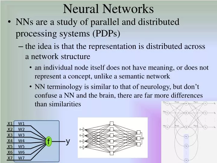
Neural Networks • NNs are a study of parallel and distributed processing systems (PDPs) • the idea is that the representation is distributed across a network structure • an individual node itself does not have meaning, or does not represent a concept, unlike a semantic network • NN terminology is similar to that of neurology, but don’t confuse a NN and the brain, there are far more differences than similarities
NN Appeal • They are trained rather than programmed • development does not entail the cost of an expert system • They provide a form of graceful degradation • if part of the representation is damaged (destroyed, removed), the performance degrades “gracefully” rather than completely as with a brittle expert system which might lack the proper knowledge • They are particularly useful at solving certain classes of problems • low-level classification/recognition • optimization • content addressable memory • Most of these problems are very difficult to solve by expert system
Inspiration from the Brain • NNs are inspired by the structure of neurons in the brain • neurons connect to other neurons by synapses • some neurons “fire” which sends electrochemical activity to neighboring neurons across synapses • if the neuron excites another neuron, then the excited neuron has a greater chance to fire – an excitation link • if the neuron inhibits another neuron, then the inhibited neuron has less of a chance to fire – an inhibition link
NNs Are Not Brains • The NN uses the idea of “spreading activation” to determine which nodes fire and which nodes do not • The NN learns whether a node should excite or inhibit another node by adjusting the edge weights on the link between them • but this analogy should not be taken too far! • NNs differ greatly in structure and learning algorithms, we will explore the earliest form for an introduction before looking at several newer and more useful forms • Many have looked to NNs as the “savior of AI” but in fact we find limited uses of most NNs • NNs can also be overtrained leading to poor performance on test data
An Artificial Neuron We need to specify or learn the weights • A neural network is a collection of artificial neurons • the neuron responds to input, in this case coming from x1, x2, …, xn • the neuron computes its output value, denoted here as f(net)
How does the Neuron Work? • First, introduce input (x1, x2, …, xn) • Second, compute f(net) • x1*w1 + x2*w2 + … + xn*wn • Third, given f(net), apply the activation function to determine if this neuron is on or off • a simple activation function is f(net) >= threshold • Fourth, provide the output of the neuron • In some cases, this will be +1 or -1, in others +1 or 0, and in others, a real number between 0 and 1
Early NNs • First proposed in 1943, the McCulloch-Pitts neuron uses the simple comparison shown on the previous slide for activation • The perceptron, introduced in 1958 is similar but has a learning algorithm so that the weights can be adjusted when training examples are used • thus, the perceptron learns the appropriate weights • By adjusting the weights with each new training instance, we are discovering the weights that cause the perceptron to output for the given input that it is or is not in the class – we are learning classification for whatever the input represents (e.g., is the input a ‘A’ or not?)
Perceptron Learning Algorithm • Let the expected output of the perceptron be di • Let the real output of the perceptron for this input be oi • Let c be some constant training weight constant • Let xj be the input value for input j • For training, repeat for each training example i • wi = (di – oi) * xi • collect all wi into a vector and then set w = w + Dw * c • that is, wi = wi + c * (di - oi) * xi for each i • Repeat the training set until the weights are not changing • Notice that dj – oj will either be +2, 0, or -2 • so in fact we will always be altering the weights by +2*c, 0*c or -2*c • Note that in a perceptron, we add an n+1st input value with a weight of 1, known as the bias
Examples • Perceptrons to learn functions X AND Y and X OR Y • weights have been pre-set • The data on the right is used to train a perceptron • to learn the class • as shown on the left
Perceptron Networks • A single perceptron can learn a simple function • We can combine perceptrons into a larger neural network that can perform a more complex task • A perceptron network is might consist of • low-level data transformer perceptrons • low level pattern matchers perceptrons • feature detectors perceptrons • classifier perceptrons • Unfortunately, the • perceptron learning • algorithm can only • train a single perceptron, • not a network of • perceptrons
Linear Separability • The data makes up points in an n-dimensional space • a perceptron learns a dividing line between data that are in the learned class and data that are not in the learned class • This only works if the division is linearly separable • in a 2-D case, it’s a simple line • in a 3-D case, it’s a plane • in a 4-D case, it’s a hyperplane • The figure to the right shows a line that separates the two sets of data
Are All Problems Linearly Separable? • The answer is no, one simple problem which is not is XOR, see the figure below • There is no single line that can separate the points where the output is 1 from the points where the output is 0! The problem is that the perceptron is learning a linear function whereas most problems comprise much more complex functions
Learning a Function • We want to learn a function which captures data • To separate those “in” from those “out” of a class • Or to learn a function which closely resembles the data • while we will probably not learn the function exactly, we hope to learn a function which approximates the function • We will come up with a cost function that computes the error that our learned function has compared to the true output of the data • our goal for our learning algorithm is to minimize this error, or the cost function We try to learn the data points given We might learn the function indicated by the green line, is this accurate enough? A more complex learning algorithm might learn the function shown by the red line which is not linear
The traditional approach to learning a function is through regression Here, the strategy is to identify the coefficients (such as a, b below) to fit the equation below, given the data set of <x, y> values e is some random element we need to expand on this to be an n-dimensional formula since our data will consist of elements X = {x1, x2, x3, …, xn}, and y There are a variety of ways to do regression some sort of distribution (e.g., Gaussian) applying the method of least squares applying Bayesian probabilities, etc Linear Regression y = α + βx + e
SVMs • The perceptron’s learning algorithm limited us to linearly separable functions, what if our data is not linearly separable? • One solution is to use the support vector machine (SVM) • Although the SVM by default learns a line, there are adjustments that can be made to the learning algorithm • given data in n dimensions (i.e., our data consists of data of n attributes), the SVM will learn a hyperplane in n-1 dimensional space that separates the positive from the negative examples • The idea is, given data x1, x2, x3, …, xn, and y (1 if in the class, -1 if not in the class) to find the vector W consisting of w1, w2, w3, …, wn such that • w o x – b = 0 (where o is the dot product)
Types of SVMs • But the SVM differs from the perceptron because we can translate the n-dimensional data into a higher dimensionality using a kernel function • Types of SVMs • Linear – linearly separable • Soft margin – a linear SVM in which the hyperplane can divide most, but not all, of the data appropriately – an approximation • Non-linear – we apply a kernel function in place of the former dot product to transform the space from n dimensions to some higher dimensionality • There are three commonly applied kernel functions (see next slide)
Kernel Functions • Polynomial: use (x o y + c)d • d is the dimensionality for the function indicating the range of types of curves that can be learned (e.g., d = 2 would allow for a parabola) • Gaussian radial basis: use e(-||x-y||2)/2p • here, we are using the “least squares” method to compute distance between each pair of points, p is some adjustable parameter • Hyperbolic tangent: use tanh(k * x o y + c) for some value k > 0 and c < 0
Multiclass SVMs • The traditional SVM recognizes data as being in or not in a single class • The multiclass SVM is used to identify the class that some data is in where there are multiple (more than 1) classes • Here, we can train multiple SVMs, one per class and then when we supply a new datum, determine which SVM outputs the highest score • Or, we can train multiple SVMs where each SVM recognizes between one of two classes – the datum is thought to be in class X if X is the class voted on most by the SVMs that compare X to other classes
Why Not SVM? • Obviously the SVM is superior to the perceptron, why should we not use the SVM? • SVMs have other advantages like not requiring an equal (or near equal) number of + and – examples in the test data and learning does not get stuck in “local minima” (we examine this later) • We might prefer a NN though because a single NN can learn multiple classes while the SVM approach requires training independent SVMs • There are also more learning algorithms for NNs which can learn a wider range of problem types than SVMs • You also have to guess a proper kernel function for the SVM to work well, that is not the case for the NN • So let’s return to NNs…
Beyond Perceptron Limitations • The perceptron can only learn linearly separable functions • We can build multi-layered perceptrons but only if we provide the weights between layers • We want to improve on this • The multi-layered feed-forward network (multiple layers of perceptrons) can learn their weights through an algorithm called back propagation • For back prop, we need to identify a cost function which will determine the error between our training set’s expected output and our FF/BP output • While we are at it, we will improve the activation function to permit uncertainty
A FF/BP Multilayered Network • Sometimes called a MLP
Threshold Functions • The perceptron provides a binary output f(net) = (x1*w1+x2*w2+…) and the output is based on whether this value >= t or not • such a function is known as a linear threshold (or a bipolar linear threshold) • We instead turn to the sigmoid function • this not only gives us “in-between” responses, but is also a continuous function, which will be important for our new training algorithm In this case, S = s * net where net is as defined before and s is a “squashing function” used for training (s may change over time)
Comparing Threshold Functions • In the sigmoid function, output is a real number between 1 and 0 • the slope increases dramatically near the threshold point but is much more shallow once you get beyond the threshold • for instance net = 0 means 1 / (1 + e-0) = ½ • net = 100 means 1 / (1 + e-100) which is nearly 1 • net = -100 means 1 / (1 + e100) which is nearly 0 a squashed sigmoid function makes the steepness more pronounced
Cost Function • As with the perceptron and SVM, we are learning the weights of the MLP • we have a lot more weights to learn, one set per node in the MLP • In order to judge how well we are learning, we develop a cost function • cost is the error given our values in our training set and the expected output • what we want to do is minimize the cost (error) • One common cost function is the Euclidean distance between the output from the MLP and the expected output • We use the cost function in order to adjust our weights for our BP algorithm
Gradient Descent Learning • Imagine the collection of weights of our MLP are plotted in an n+1 dimensional space where one axis is the error rate • Our learning algorithm will adjust the weights so that we move toward the minimum error • this is a process called gradient descent • For the perceptron and SVM, we are guaranteed of finding the global minima (the least error) • For a FF/BP MLP, we are not guaranteed this and so we might find ourselves descending to a local minimum • In such a case, we may wind up learning the training data so that our MLP is overfitted to that data and does not respond well to the testing data • There are various ways to try to avoid being stuck in a local minimum
Delta Rule • The delta rule is the formula we will use to update our edge weights • The idea is that wi,j will be modified by adding to it the value of c * (di – Oi) * f’(neti) xj • c is the constant training rate of adjustment • di is the value we expect out of the given node i • Oi is the actual output of the given node i • f is the threshold function so f’ is its partial derivative • xj is the jth input into the given node i • Notice that we need to compute the derivative f • This is one reason why we had to change activation functions, the binary activation function’s derivative will be 0 in all cases except when net = 0 in which case the derivative doesn’t exist!
Training • For each item in the training set • Feedforward from input to output layer through all hidden layers • Compute what the output should have been (this should be part of the data set) • Use this error to backprop to previous layer, adjusting weights (between last hidden layer and output layer) • Compute error for hidden layer nodes and continue to back propagate errors to prior levels until you reach the weights between first hidden layer and input • Repeat until training set is complete • if the edge weights have not reached a stable state, repeat
Output to Hidden Layer • Compute the error for the edge weight from node k to output i to readjust the weight • weightki = weightki + -c * (di – Oi) * Oi * (1 – Oi) * xk • c is the training constant • di is the expected value of the output node i • Oi is the actual value computed for node i • xk is the value of node xkfrom the previous layer • We can directly compute the error between these two layers because we know the expected output (Oi) versus the actual output (di) • that is, we expect a particular output node to be 1 and all others to be 0
The Hidden Layer Nodes • What about correcting the edge weights leading to hidden layer nodes? • we do not have a similar “expected” value for a hidden layer node because the hidden layer nodes do not represent anything that we can understand • input nodes represent whether an input feature is present or not • output nodes represent the final value of the network (for instance, which of n classes the input was classified as) • but hidden layer nodes don’t represent anything specifically
Training a Hidden Layer Node • For a hidden layer node i, we adjust the weight from node k of the previous (lower) level as • wik = wik + -c * Oi * (1 – Oi) * Sumj (- deltaj * wij) * xk • where Sumj adds up all of the errors * edge weights of edges coming out of node i to the next level • -deltaj is the error from the jth node in the next level that this node connects too and is really f’(netj) where f is the delta rule • note that the minus signs in -c and -delta will cancel giving us • wik = wik + c * Oi * (1 – Oi) * Sumj (deltaj * wij) * xk
Training the NN • The NN requires dozens to hundreds of training examples • one iteration through the entire training set is called an epoch • it usually takes hundreds or thousands of epochs to train a NN (with 50 training examples, if it takes 1,000 epochs for edge weights to converge, then you would run the algorithm 20,000 times! • The MLP training time is deeply affected by initial conditions: size, shape, initial weights • The figure to the right demonstrates training a 2x2x1 NN to compute XOR using different starting conditions where the shade of grey represent approximate number of epochs required
Unsupervised Learning • All of the previous approaches (perceptron, SVM, FF/BP MLP) were forms of supervised learning • Each training example included the expected result (the class that it belong to) • ANNs can be used for unsupervised learning to solve very different types of problems • In this case, we do not have an output to derive the error via a cost function, so our cost function must be based on something other than error • The cost function we will select will be based on the type of operation that we are trying to learn • compression – a comparative size between x and f(x) • clustering – some statistical distribution
Competitive Learning • Here, we want to compute f(x) for a given x and then adjust weights so that the same f(x) output will result from x and input similar to x • We use a “winner-take-all” form of learning • Introduce an example, the output node with the highest value is judged the “winner” • edge weights from node i to this output node are adjusted by c*(xi – wi) • c is our training constant • xi is the value of input node i • wi is the previous edge weight from node i to this node • If input patterns differ sufficiently, different output nodes will be strengthened for different types of inputs • this type of NN is called a self-organizing network (or map), often referred to as a Kohonen network
Kohonen Network • These networks do not include hidden layers • input maps directly to output • 1 output per type of category that we want to learn • Initialize weights at random and repeat until weights do not change much between iterations • For each datum, X (x1, x2, x3, …) • Compute the output and select the winner • Modify the weights for all inputs j to winning node i using the wi,j = wi,j + a* (xj – wi,j) • a is a training constant • We might use this for clustering (finding groupings of data that are “near” to each other), filtering and computing statistical distributions
Clustering Example • Using the data from our previous clustering example • the Kohonen network to the left learns to classify the data clusters as prototype 1 (node A) and prototype 2 (node B) • over time, the network organizes itself so that one node represents one cluster and the other node represents the other cluster
Reinforcement Learning • There is less literature on reinforcement learning with NNs but here are two possible approaches • Given a MLP FF/BP network, generate input based on the actions of the entity being modeled (e.g., a process, a robot) • The output is an action which is performed and stored along with the effort it takes the entity to perform the operation • based on the utility of this operation, if it is perceived as too expensive, reduce weights that led to this output node and if it is deemed a good solution, increase the edge weights (thus it is similar to backprop) • as time goes on, alter the NN’s hidden layer nodes (add a node with new random weights) and see how this compares to the efficiency of the operation previously
Hebbian Learning • Hebb’s theory states that neurons that repeatedly activate at the same time tend to become ‘associated’ with each other • In NNs, a Hebbian network is one where weights between two nodes model how associated they should be (whether they should both fire or not) • We might implement Hebbian learning in a network where we want to develop coincedence-based learning such as condition-responses • In this type of learning, there are two sets of inputs • the first set is a condition that should elicit the desired response • the second set of inputs is a second condition that needs to learn the same response as the first set of inputs
Hebbian Network • In this example, the top three inputs represent the initial condition that we learn first • Once learned, the task is for the network to learn the weights for the bottom three inputs so that a different input condition will elicit the same output response
Supervised Hebbian Learning • We want a network to learn associations • Use a single layered, fully connected network where n inputs map directly to m outputs • We do not train our edge weights, instead we compute them using a simple vector dot product of the training examples • the formula to determine the edge weight from input i to output k is Dwik= c * dk * xi • where c is our training constant • dk is the desired output of the kth output node and xi is the ith input • We can compute a vector to adjust all weights as once with • DW = c * Y * X • where W is the vector of weights and Y * X is the outer product of a matrix that stores the associations (see the next slide)
Example • We have the following two associations • [1, -1, -1, -1] [-1, 1, 1] • [-1, -1, -1, 1] [1, -1, 1] • That is, input of x1 = 1, x2 = -1, x3 = -1 and x4 = -1 should provide the output of y1 = -1, y2 = 1, y3 = 1 • The resulting network is shown to the right – notice every weight is either +2, 0 or -2 • this is computed using the matrix sum shown to the right
Unsupervised Hebbian Learning • Assume a network is already trained on the initial condition using supervised learning • Now we introduce a second condition • the first set of edge weights are stable, we will not adjust those • the second set of edge weights are initialized randomly (or to all 0s) • With the new data set, we only modify the second set of edge weights • using the formula: wi = wi + c * f(X, W) * xi • wi is the current edge weight • c is the training constant • f(X, W) is the output of the node (a +1 or a -1) • xi is the input value • We are altering the latter set of edge weights to respond in the same way as the first set of edge weights but without using the training data results
Attractor Networks • The preceding forms of NNs were all feed-forward types • given input, values are propagated forward to compute the result • A Bi-directional Associative Memory (BAM) consists of bi-directional edges so that information can flow in either direction • nodes can also have recurrent edges
Using a BAM Network • Propagation moves in both directions, first from one layer to another, and then back to the first layer • edge weights are bidirectional, wij = wji for all edges • The propagation can be done sequentially, node by node, or in parallel • Propagation continues until the nodes are stable • We use BAM networks as attractor networks which provide a form of content addressable memory • given an input, we reach the nearest stable state • Edge weights are worked out in advance without training by computing a vector matrix
Using a BAM Network • Introduce an input and propagate to the other layer • a node’s activation (state) will be • = 1 if its activation function value > 0 • stay the same state if its activation function value = 0 • = -1 if its activation function value < 0 • take the activation values (states) of the computed layer and use them as input and feed back into the previous layer to modify those nodes’ states • repeat until a full iteration occurs where no node changes state – this is a stable state – the output is whatever the non-input layer values are indicating • Notice that we have moved from FF/BP training to FF/BP activations for this form of network
Hopfield Network • This is a form of BAM network • in the example below, the network has four stable states • no matter what input is introduced, the network will settle into one of these four states • the idea is that this becomes a content addressable, or autoassociative memory • the stable state we reach is whatever state is “closest” to the input • closest here is not defined by Hamming distance but instead by minimal energy – the least amount of work to reach a stable state The network to the right starts with the left-most three nodes activated and stabilizes into the state on the right – there are 4 total stable states
Hopfield Network Learning • Use a Hebbian-form of learning requiring both • Local learning – a node’s weights are modified based on information of the node’s neighbors • Incremental learning – learning a new pattern does not require information about previously learned patterns • Hebbian learning rule – weight from node i to j (and j to i) where the term eiej is positive if nodes i and j are both found in the given pattern being learned and negative otherwise
Use of a Hopfield Network • The best example is to find the closest matching pattern to a given input • this allows the network to handle some amount of graceful degradation • Hopfield networks sound great but there are drawbacks – they are not guaranteed to converge to the correct pattern and the number of nodes of the network grows rapidly to the number of patterns it must learn
Boltzmann Machines • A variation of the Hopfield network • A fully connected network where some select nodes are “hidden” nodes and the rest are input • Unlike Hopfield networks, the activation of a node is not based solely on a computation but is also probabilistic • Like Hopfield networks, the associative memory would be able to complete a partial input • However, there are many practical problems with Boltzmann machine learning, particularly for any “real-world” sized network A restrictive Boltzmann machine that doesn’t suffer as badly
Recurrent Networks • One problem with NNs as presented so far is that the input represents a “snapshot” of a situation • what happens if the situation is dynamic or where one state can influence the next state? • in speech recognition, we do not merely want to classify a sound based on this time slice of acoustic data, we need to also feed in the last state because it can influence this sound • in a recurrent network, we take or ordinary multi-layered FF/BP network and wrap the output nodes into some of (or all of) the input nodes • in this way, some of the input nodes represent “the last state” and other input nodes represent “the input for the new state”


