Download
1 / 58
610 likes | 1.07k Vues
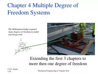
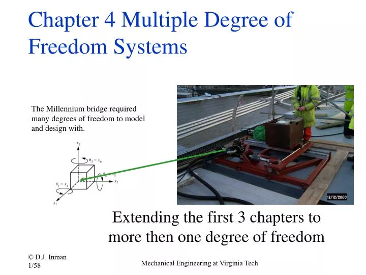
Chapter 4 Multiple Degree of Freedom Systems. The Millennium bridge required many degrees of freedom to model and design with. Extending the first 3 chapters to more then one degree of freedom. The first step in analyzing multiple degrees of freedom (DOF) is to look at 2 DOF.

E N D
Chapter 4 Multiple Degree of Freedom Systems The Millennium bridge required many degrees of freedom to model and design with. Extending the first 3 chapters to more then one degree of freedom Mechanical Engineering at Virginia Tech
The first step in analyzing multiple degrees of freedom (DOF) is to look at 2 DOF • DOF: Minimum number of coordinates to specify the position of a system • Many systems have more than 1 DOF • Examples of 2 DOF systems • car with sprung and unsprung mass (both heave) • elastic pendulum (radial and angular) • motions of a ship (roll and pitch) Fig 4.1 Mechanical Engineering at Virginia Tech
4.1 Two-Degree-of-Freedom Model (Undamped) A 2 degree of freedom system used to base much of the analysis and conceptual development of MDOF systems on. Mechanical Engineering at Virginia Tech
Free-Body Diagram of each mass Figure 4.2 k2(x2 -x1) m2 k1 x1 m1 x2 x1 Mechanical Engineering at Virginia Tech
Summing forces yields the equations of motion: Mechanical Engineering at Virginia Tech
Note that it is always the case that • A 2 Degree-of-Freedom system has • Two equations of motion! • Two natural frequencies (as we shall see)! Mechanical Engineering at Virginia Tech
The dynamics of a 2 DOF system consists of 2 homogeneous and coupled equations • Free vibrations, so homogeneous eqs. • Equations are coupled: • Both have x1 and x2. • If only one mass moves, the other follows • Example: pitch and heave of a car model • In this case the coupling is due to k2. • Mathematically and Physically • If k2 = 0, no coupling occurs and can be solved as two independent SDOF systems Mechanical Engineering at Virginia Tech
Initial Conditions • Two coupled, second -order, ordinary differential equations with constant coefficients • Needs 4 constants of integration to solve • Thus 4 initial conditions on positions and velocities Mechanical Engineering at Virginia Tech
Solution by Matrix Methods The two equations can be written in the form of a single matrix equation (see pages 272-275 if matrices and vectors are a struggle for you) : (4.4), (4.5) (4.6), (4.9) Mechanical Engineering at Virginia Tech
Initial Conditions IC’s can also be written in vector form Mechanical Engineering at Virginia Tech
The approach to a Solution: For 1DOF we assumed the scalar solution aeltSimilarly, now we assume the vector form: (4.15) (4.16) (4.17) Mechanical Engineering at Virginia Tech
This changes the differential equation of motion into algebraic vector equation: Mechanical Engineering at Virginia Tech
The condition for solution of this matrix equation requires that the the matrix inverse does not exist: The determinant results in 1 equation in one unknown w(called the characteristic equation) Mechanical Engineering at Virginia Tech
Back to our specific system: the characteristic equation is defined as (4.20) (4.21) Eq. (4.21) is quadratic inw2so four solutions result: Mechanical Engineering at Virginia Tech
Once is known, use equation (4.17) again to calculate the corresponding vectors u1 and u2 This yields vector equation for each squared frequency: Each of these matrix equations represents 2 equations in the 2 unknowns components of the vector, but the coefficient matrix is singular so each matrix equation results in only 1 independent equation. The following examples clarify this. Mechanical Engineering at Virginia Tech
Examples 4.1.5 & 4.1.6:calculating u and • m1=9 kg,m2=1kg, k1=24 N/m and k2=3 N/m • The characteristic equation becomesw4-6w2+8=(w2-2)(w2-4)=0w2 = 2 and w2 =4 or Each value of w2 yields an expression or u: Mechanical Engineering at Virginia Tech
Computing the vectors u 2 equations, 2 unknowns but DEPENDENT! (the 2nd equation is -3 times the first) Mechanical Engineering at Virginia Tech
Only the direction of vectors u can be determined, not the magnitude as it remains arbitrary Mechanical Engineering at Virginia Tech
Likewise for the second value of w2: Note that the other equation is the same Mechanical Engineering at Virginia Tech
What to do about the magnitude! Several possibilities, here we just fix one element: Choose: Choose: Mechanical Engineering at Virginia Tech
Thus the solution to the algebraic matrix equation is: Here we have introduce the name mode shape to describe the vectors u1 and u2. The origin of this name comes later Mechanical Engineering at Virginia Tech
Return now to the time response: We have computed four solutions: (4.24) Since linear, we can combine as: (4.26) Note that to go from the exponential form to to sine requires Euler’s formula for trig functions and uses up the +/- sign on omega determined by initial conditions. Mechanical Engineering at Virginia Tech
Physical interpretation of all that math! • Each of the TWO masses is oscillating at TWO natural frequenciesw1 and w2 • The relative magnitude of each sine term, and hence of the magnitude of oscillation of m1 and m2 is determined by the value of A1u1 and A2u2 • The vectors u1 and u2 are called mode shapesbecause the describe the relative magnitude of oscillation between the two masses Mechanical Engineering at Virginia Tech
What is a mode shape? • First note that A1, A2, f1 and f2 are determined by the initial conditions • Choose them so that A2 = f1 = f2 =0 • Then: • Thus each mass oscillates at (one) frequency w1 with magnitudes proportional to u1 the 1stmode shape Mechanical Engineering at Virginia Tech
A graphic look at mode shapes: If IC’s correspond to mode 1 or 2, then the response is purely in mode 1 or mode 2. x1 x2 k1 k2 m1 m2 Mode 1: x2=A x1=A/3 x1 x2 k1 k2 m1 m2 Mode 2: x2=A x1=-A/3 Mechanical Engineering at Virginia Tech
Example 4.1.7 given the initial conditions compute the time response Mechanical Engineering at Virginia Tech
At t=0 we have Mechanical Engineering at Virginia Tech
4 equations in 4 unknowns: Yields: Mechanical Engineering at Virginia Tech
The final solution is: (4.34) These initial conditions gives a response that is a combination of modes. Both harmonic, but their summation is not. Figure 4.3 Mechanical Engineering at Virginia Tech
Solution as a sum of modes Determines how the second frequency contributes to the response Determines how the first frequency contributes to the response Mechanical Engineering at Virginia Tech
Things to note • Two degrees of freedom implies two natural frequencies • Each mass oscillates at with these two frequencies present in the response and beats could result • Frequencies are not those of two component systems • The above is not the most efficient way to calculate frequencies as the following describes Mechanical Engineering at Virginia Tech
Some matrix and vector reminders Then M is said to be positive definite Mechanical Engineering at Virginia Tech
4.2 Eigenvalues and Natural Frequencies • Can connect the vibration problem with the algebraic eigenvalue problem developed in math • This will give us some powerful computational skills • And some powerful theory • All the codes have eigen-solvers so these painful calculations can be automated Mechanical Engineering at Virginia Tech
Some matrix results to help us use available computational tools: A matrix M is defined to be symmetric if A symmetric matrix M is positive definite if A symmetric positive definite matrix M can be factored Here L is upper triangular, called a Cholesky matrix Mechanical Engineering at Virginia Tech
If the matrix L is diagonal, it defines the matrix square root Mechanical Engineering at Virginia Tech
A change of coordinates is introduced to capitalize on existing mathematics For a symmetric, positive definite matrix M: Mechanical Engineering at Virginia Tech
How the vibration problem relates to the real symmetric eigenvalue problem Mechanical Engineering at Virginia Tech
Important Properties of the n x n Real Symmetric Eigenvalue Problem • There are n eigenvalues and they are all real valued • There are n eigenvectors and they are all real valued • The set of eigenvectors are orthogonal • The set of eigenvectors are linearly independent • The matrix is similar to a diagonal matrix Window 4.1 page 285 Mechanical Engineering at Virginia Tech
Square Matrix Review • Let aik be the ikth element of A then A is symmetric if aik = aki denoted AT=A • A is positive definite if xTAx > 0 for all nonzero x (also implies each li > 0) • The stiffness matrix is usually symmetric and positive semi definite (could have a zero eigenvalue) • The mass matrix is positive definite and symmetric (and so far, its diagonal) Mechanical Engineering at Virginia Tech
Normal and orthogonal vectors (4.43) Mechanical Engineering at Virginia Tech
Normalizing any vector can be done by dividing it by its norm: (4.44) To see this compute Mechanical Engineering at Virginia Tech
Examples 4.2.2 through 4.2.4 Mechanical Engineering at Virginia Tech
The first normalized eigenvector Mechanical Engineering at Virginia Tech
Likewise the second normalized eigenvector is computed and shown to be orthogonal to the first, so that the set is orthonormal Mechanical Engineering at Virginia Tech
Modes u and Eigenvectors v are different but related: (4.37) Mechanical Engineering at Virginia Tech
This orthonormal set of vectors is used to form an Orthogonal Matrix called a matrix of eigenvectors (normalized) P is called an orthogonal matrix (4.47) P is also called a modal matrix Mechanical Engineering at Virginia Tech
Example 4.2.3 compute P and show that it is an orthogonal matrix From the previous example: Mechanical Engineering at Virginia Tech
Example 4.2.4 Compute the square of the frequencies by matrix manipulation In general: Mechanical Engineering at Virginia Tech
Example 4.2.5 The equations of motion: Figure 4.4 In matrix form these become: Mechanical Engineering at Virginia Tech
Next substitute numerical values and compute P and Mechanical Engineering at Virginia Tech