Download
1 / 27
280 likes | 813 Vues
Descriptive Statistics Healey Chapters 3 and 4 (2 nd Cdn Ch. 3). Measures of Central Tendency And Dispersion. Measures of Central Tendency. 1. Mode = can be used for any kind of data but only measure of central tendency for nominal or qualitative data.

E N D
Descriptive StatisticsHealey Chapters 3 and 4(2nd Cdn Ch. 3) Measures of Central Tendency And Dispersion
Measures of Central Tendency • 1. Mode = can be used for any kind of data but only measure of central tendency for nominal or qualitative data. • Formula: value that occurs most often or the category or interval with highest frequency. • Note: Omit Formula 3.1 Variation Ratio in Healey and Prus 2nd Cdn.
Example for Nominal Variables: • Religion frequency cf proportion % Cum% • Catholic 17 17 .41 41 41 • Protestant 4 21 .10 10 51 • Jewish 2 23 .05 5 56 • Muslim 1 24 .02 2 58 • Other 9 33 .22 9 80 • None 8 41 .20 20 100 • Total 41 1.00 100% • Central Tendency: MODE = largest category = Catholic
Central Tendency (cont.) • 2. Median = exact centre or middle of ordered data. The 50th percentile. • Formula: • Array data. • When sample even #, median falls halfway between two middle numbers. • To calculate: find(n/2)and (n/2)+1, and divide the total by 2 to find the exact median. • When sample is odd #, median is exact middle (n+1) /2)
Example for Raw Data: • Suppose you have the following set of test scores: • 66, 89, 41, 98, 76, 77, 69, 60, 60, 66, 69, 66, 98, 52, 74, 66, 89, 95, 66, 69 • 1. Array data: • 98 98 95 89 89 77 76 74 69 69 69 66 66 66 66 66 60 60 52 41 N = 20 (N is even)
To calculate: - find middle numbers(n/2)+(n/2 )+1- add together the two middle numbers- divide the total by 2 • First middle number: (20/2) = the 10th number • 2nd middle number: (20/2)+1 = the 11th • Look at data: the middle numbers are 69 and 69 The median would be (69+69)/2 = 69
Median for Aggregate (grouped) Data • This formula is shown in Healey 1st Cdn Edition and in Healey 8e but NOT in 2nd Cdn • We will NOT COVER this one!
Properties of median: • - for numerical data at interval or ordinal level • -"balance point“ • -not affected by outliers • -median is appropriate when distribution is highly skewed.
3. Mean for Raw Data • The mean is the sum of measurements / number of subjects • Formula: (X-bar) = ΣXi / N • Data (from above): 66, 89, 41, 98, 76, 77, 69, 60, 60, 66, 69, 66, 98, 52, 74, 66, 89, 95, 66, 69
Example for Mean • Formula: = ΣXi / N = 1446 / 20 = 72.3 The mean for these test scores is 72.3
Mean for Aggregate (Grouped) Data(Note: 1st Cdn. Edition: use this formula! Omitted in 2nd Cdn. Ed. but covered in class) • To calculate the mean for grouped data, you need a frequency table that includes a column for the midpoints, for the product of the frequencies times the midpoints (fm). Formula: = Σ (fm) N
Frequency table: Score f m* (fm) 41-50 1 45.5 45.5 51-60 3 55.5 166.5 61-70 8 65.5 524 71-80 3 75.5 226.5 81-90 2 85.5 171 91-100 3 95.5 286.5 N = 20 Σ (fm) = 1420 * Find midpoints first
Calculating Mean for Grouped Data: Formula: = Σ (fm) N = 1420 / 20 = 71 The mean for the grouped data is 71.
Properties of the Mean: - only for numerical data at interval level - "balance point“ - can be affected by outliers = skewed distribution - tail becomes elongated and the mean is pulled in direction of outlier. Example… no outlier: $30000, 30000, 35000, 25000, 30000 then mean = $30000 but if outlier is present, then: $130000, 30000, 35000, 25000, 30000 then mean = $50000 (the mean is pulled up or down in the direction of the outlier)
NOTE: • When distribution is symmetric, mean = median = mode • For skewed, mean will lie in direction of skew. • i.e. skewed to right, mean > median (positive skew) • skewed to left, median > mean (negative skew)
Measures of Dispersion • Describe how variable the data are. • i.e. how spread out around the mean • Also called measures of variation or variability
Variability for Non-numerical Data (Nominal or Ordinal Level Data) • Measures of variability for non-numerical nominal or ordinal) data are rarely used • We will not be covering these in class • Omit Formula 4.1 IQV in Healey and Prus 1st Canadian Edition and in Healey 8e • Omit Formula 3.1 Variation Ratio in Healey and Prus 2nd Canadian Edition
2. Range (for numerical data) Range = difference between largest and smallest observations i.e. if data are $130000, 35000, 30000, 30000, 30000, 30000, 25000, 25000 then range = 130000 - 25000 = $105000
Interquartile Range (Q): • This is the difference between the 75th and the 25th percentiles (the middle 50%) • Gives better idea than range of what the middle of the distribution looks like. Formula: Q = Q3 - Q1 (where Q3 = N x .75, and Q1 = N x .25) Using above data: Q = Q3 - Q1 = (6th – 2nd case) = $30000-25000 =$5000 The interquartile range (Q) is $5000.
3. Variance and Standard Deviation: • For raw data at the interval/ratio level. • Most common measure of variation. • The numerator in the formula is known as the sum of squares, and the denominator is either the population size N or the sample size n-1 • The variance is denoted by S2 and the standard deviation, which is the square root of the variance, by S
Definitional Formula for Variance and Standard Deviation: • Variance: s2 = Σ (xi - )2 / N • S.D.: s = • A working formula (the one you use) for s.d is: 1 N ∑ Xi2 - ( ∑ Xi ) 2 N
Example for S and S2 : • Data: 66, 89, 41, 98, 76, 77, 69, 60, 60, 66, 69, 66, 98, 52, 74, 66, 89, 95, 66, 69 • Find ∑ Xi2 : Square each Xi and find total. • Find (∑ Xi)2 : Find total of all Xi and square. • Substitute above and N into formula for S. • For S2 , simply square S. S = 14.76 S2 = 217.91
Another working formula for the standard deviation: Note that the definitional formula for s.d. is not practical for use with data when N>10. The working formulae should be used instead. All three formulae give exactly the same result.
Properties of S: • always greater than or equal to 0 • the greater the variation about mean, the greater S is • n-1 (corrects for bias when using sample data.) S tends to underestimate the population s.d. so to correct for this, we use n-1. The larger the sample size, the smaller difference this correction makes. When calculating the s.d. for the whole population, use N in the denominator.
NOTE: • σ, N and Mu (µ) denote population parameters • s, n, x-bar ( ) denote sample statistics
Remember the Rounding Rules! • Always use as many decimal places as your calculator can handle. • Round your final answer to 2 decimal places, rounding to nearest number. • Engineers Rule: When last digit is exactly 5 (followed by 0’s), round the digit before the last digit to nearest EVEN number.
Homework Questions • Healey and Prus 1st Cdn. And Healey 8e: • #3.1, #3.5, #3.11 and 4.9, #4.15 • Healey and Prus 2nd Cdn. • #3.1, #3.5, #3.11 (compute s for 8 nations also), #3.15 • SPSS: • Read the SPSS sections for Ch. 3 and 4 in 1st Cdn. Edition and for Ch. 4 in 2nd Cdn. Edition • Try some of the SPSS exercises for practice