Download

1 / 57
580 likes | 768 Vues
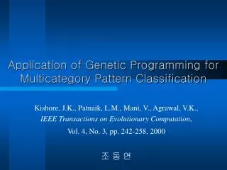
The Application Of Genetic Programming. lujing. Contents:. Time Series Forecasting for Dynamic Environments : The DyFor Genetic Program Model Forecasting time series using a methodology based on autoregressive integrated moving average and genetic programming

E N D
Contents: • Time Series Forecasting for Dynamic Environments : The DyFor Genetic Program Model • Forecasting time series using a methodology based on autoregressive integrated moving average and genetic programming • Forecasting nonlinear time series of energy consumption using a hybrid dynamic model • Genetic programming-based voice activity detection
1、Time Series Forecasting for Dynamic Environments : The DyFor Genetic Program Model • Abstract • Review Of Existing Time Series Forecasting Methods • The DYFOR GP Model
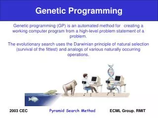
1.1Abstract: Several studies have applied genetic programming (GP) to the task of forecasting with favorable results. However,these studies, like those applying other techniques, have assumed a static environment.
If a time series is produced in a nonstatic environment, frequently only the recent historical data that correspond to the current environment are analyzed and historical data that come from previous environments are ignored.
This study investigates the development of a new “dynamic” GP model that is specifically tailored for forecasting in nonstatic environments. • This Dynamic Forecasting Genetic Program (DyFor GP) model incorporates features that allow it to adapt to changing environments automatically as well as retain knowledge learned from previously encountered environments.
The DyFor GP model is tested for forecasting efficacy on both simulated and actual time series including the U.S. Gross Domestic Product and Consumer Price Index Inflation.
1.2 REVIEW OF EXISTING TIME SERIES FORECASTING METHODS • Classical Methods: 1) exponential smoothing methods; 2) regression methods; 3) autoregressive integrated moving average (ARIMA)methods; 4) threshold methods; 5) generalized autoregressive conditionally heteroskedastic (GARCH) methods.
Modern Heuristic Methods: 1) methods based on neural networks (NNs); 2) methods based on evolutionary computation(GP).
1.3 THE DYFOR GP MODEL • As discussed in Section II, existing forecasting methods rely, to some degree, on human judgment to designate an appropriate analysis window (i.e., the correct number of historical data to be analyzed).
Consider the following example. Suppose the time series given in Fig. 4 is to be analyzed and forecast.
As depicted in the figure, this time series consists of two segments each with a different underlying data generating process. • The first segment’s process represents an older environment that no longer exists but may contain patterns that can be learned and exploited when forecasting the current environment. • The second segment’s underlying process represents the current environment and is valid for forecasting future data.
This is accomplished in the following way. • 1) Select two initial window sizes, one of size n and one of size n+i , where n and i are positive integers. • 2) Run dynamic generations at the beginning of the historical data with window sizes n and n+i , use the best solution for each of these two independent runs to predict a number of future data points, and measure their predictive accuracy.
3) Select another two window sizes based on which window size had better accuracy. For example, if the smaller of the two window sizes (size n) predicted more accurately, then choose two new window sizes, one of size n and one of size n-i. If the larger of the two window sizes (size n+i) predicted more accurately, then choose window sizes n+i and n+2i.
4) Slide the analysis window to include the next time series observation. Use the two selected window sizes to run another two dynamic generations, predict future data, and measure their prediction accuracy. • 5) Repeat the previous two steps until the analysis window reaches the end of historical data.
However , after several window slides, when the data analysis window spans data from both the first and second segments, it is likely that the window adjustment reverses direction. Figs. 7 and 8 show this phenomenon.
In Fig. 7, win1 and win2 have sizes of 4 and 5, respectively. As the prediction data, pred lies inside the second segment, it is likely that the dynamic generation involving analysis window win1 has better prediction accuracy than that involving win2 because win1 includes less data produced by a process that is no longer in effect. If this is so, the two new window sizes selected for win1 and win2 are sizes 3 and 4, respectively. Thus, as the analysis window slides to incorporate the next time series value, it also contracts to include a smaller number of inappropriate data. In Fig. 8, this contraction is shown.
After the data analysis window slides past the end of the first segment, it is likely to expand again to encompass a greater number of appropriate data. Figs. 9 and 10 depict this expansion.
As illustrated in the above example, the DyFor GP uses predictive accuracy to adapt the size of its analysis window automatically. • When the underlying process is stable (i.e., the analysis window is contained inside a single segment), the window size is likely to expand. • When the underlying process shifts (i.e., the analysis window spans more than one segment), the window size is likely to contract.
2、Forecasting time series using a methodology based on autoregressive integrated moving average and genetic programming • Abstract • ARIMA Model • Hybrid Forecasting Model • The Model Development
2.1 Abstract • The autoregressive integrated moving average (ARIMA), which is a conventional statistical method, is employed in many fields to construct models for forecasting time series. Although ARIMA can be adopted to obtain a highly accurate linear forecasting model, it cannot accurately forecast nonlinear time series.
This study proposes a hybrid forecasting model for nonlinear time series by combining ARIMA with genetic programming (GP). Finally, some real data sets are adopted to demonstrate the effectiveness of the proposed forecasting model.
2.2 ARIMA Model • Box and Jenkins presented the ARIMA model in 1970.The method has been widely used in financial, economic and social scientific fields. • In the ARIMA(p, d, q) model, p is the order of auto-regression, d is the order of differencing, and q is the order of the moving average process. • Generally speaking, the ARIMA model can be represented as a linear combination of the past observations and past errors as follows:
where is the actual value, B is the backward shift operator, is the constant item, is the random error at time t, and are the coefficients of the model and can be estimated utilizing the least square method.
2.3 Hybrid Forecasting Model • Several investigations have developed some hybrid forecasting models that combine different methods to reduce the forecast error.
The hybrid models can be expressed as follows: where represents the original positive time series at time t; represents the linear component, and is the nonlinear component of the model, respectively. (1)
The residuals can be obtained using the ARIMA model: • where is estimated using such nonlinear methods as GP. is the forecasted value of and is estimated using the ARIMA model. (2)
Accordingly, the residual can be rewritten as follows: • where represents the nonlinear function that is constructed using GP and is the random error term. The hybrid model for forecasting time series is: (3) (4)
2.4 The model development • This study proposes a novel hybrid forecasting model, which combines ARIMA to model the linear component ( )of a time series and the GP to model the nonlinear component ( ), to improve the accuracy of ARIMA forecasting.
The proposed hybrid approach is as follows: • Step 1: The ARIMA model is utilized to model the linear component of time series. That is, is obtained by using the ARIMA model. • Step 2: From Step 1, the residuals from the ARIMA model can be obtained. The residuals are modeled by the GP model in Eq. (3).That is, is the forecast value of Eq. (3) by using GP. • Step 3: Using Eq. (4), forecasts of the hybrid model are obtained by adding the forecasted values of linear and nonlinear components , yield in Step 1 and Step 2, respectively.
3、Forecasting nonlinear time series of energy consumption using a hybrid dynamic model • Abstract • Energy Consumption Models • Hybrid Dynamic Grey Forecasting
3.1 Abstract • Energy consumption is an important index of the economic development of a country. Rapid changes in industry and the economy strongly affect energy consumption. • Although traditional statistical approaches yield accurate forecasts of energy consumption, they may suffer from several limitations such as the need for large data sets and the assumption of a linear formula. • This work describes a novel hybrid dynamic approach that combines a dynamic grey model with genetic programming to forecast energy consumption.
3.2 Energy Consumption Models 3.2.1. GM(1,1) forecasting model This model can be constructed as follows: Step 1: Obtain positive time-series data as follows: Step 2: Apply the accumulated generating operator (AGO) to the original time-series data (i.e. ) to obtain the accumulated time-series as follows: Where
Step 3: Construct GM(1,1) using a grey differential equation, where a and u denote the grey parameters of the GM(1,1) model, and represents the average of and . Also, the grey parameters of the grey differential equation can be estimated using the ordinary least squares (OLS) method.
Step4:Replace the estimated parameters ( and ) in the grey differential equation and then obtain the GM(1,1) forecasting equation using the inverse AGO (IAGO) technique, in the following exponential form.
3.2.2. Dynamic GM(1,1) model • Some studies have developed dynamic GM(1,1) models (DGM(1,1)) to increase the forecasting accuracy of GM(1,1). • In the DGM(1,1) model, is predicted using GM(1,1) and where k < n. Following the determination of , is added to the original time-series, and is removed from the original time-series to yield a new series
The predicted value of can be obtained using the new series . • The evaluation procedure is continued to obtain for l=3,4,5,…, n -k -1.
3.3 Hybrid Dynamic Grey Forecasting • This section describes a novel nonlinear hybrid dynamic forecasting model that combines the dynamic grey model with GP. The proposed model is derived as follows:
Step 1: Assume that original time-series of energy consumption data is (n data points), and that is predicted using a novel DGM(1,1) model (NDGM(1,1)). Because GM(1,1) requires at least four data points to construct the forecasting model, Therefore, in the first rolling, can be determined from the series
In the second rolling, can be determined from • Moreover, in each rolling cycle, the newly predicted values of original data are determined using the GM(1,1) model. The residual series of the NDGM (1,1) model can be expressed .
Step 2: In each rolling cycle of NDGM(1,1), construct the model for forecasting the error using the nonlinear function , determined by GP as follows: • where denotes the jth point estimate of NDGM(1,1) that is conditioned in the ith rolling cycle; the series represents the errors of the ith rolling cycle and can be obtained using the GM(1,1) model in the four periods; represents a random error.
In the GP model, the input variables are the lagging residual series and the output variable is . • To reduce the forecasting error, the fitness function in GP is defined as follows :
Step 3: Express the hybrid dynamic forecasting model that combines the NDGM(1,1) model and the GP model as follows. • where denotes the forecasted value of y; represents the series ; and represents the series
4、Genetic programming-based voice activity detection • Abstract • Definition of GP-VAD algorithm
4.1 Abstract • A voice activity detector (VAD) is a classifier the output of which is 1 or 0 indicating, respectively, the presence of voice or silence (noise) in each speech frame • A voice activity detection (VAD) algorithm is generated by using genetic programming (GP). The inputs of this VAD are the parameters extracted from the speech signals according to the ITU-T G.729B VAD standard. • The GP-based VAD algorithm (GP-VAD) is evaluated using the AURORA-2 database.
4.2Definition of GP-VAD algorithm • GP-VAD employs the same five parameters extracted by G.729B within each 10 ms frame : • the full-band energy, ; • full-band energy difference, ; • low-band energy difference, ; • zero-crossing rate difference, ; • the spectral distortion, . • Let Y(n) be the GP-VAD decision at frame n. The previous decisions Y(n-1) and Y(n-2) are also incorporated as inputs.
For the GP-VAD approach, the five preparatory steps mentioned above were defined as follows: • Function set. • Terminal set. • Fitness measure. • Control parameters. • The termination criterion