Download
1 / 15
250 likes | 618 Vues
Conjugate gradient iteration. x 0 = 0, r 0 = b, d 0 = r 0 for k = 1, 2, 3, . . . α k = (r T k-1 r k-1 ) / (d T k-1 Ad k-1 ) step length x k = x k-1 + α k d k-1 approx solution

E N D
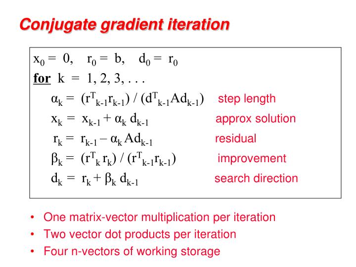
Conjugate gradient iteration x0 = 0, r0 = b, d0 = r0 for k = 1, 2, 3, . . . αk = (rTk-1rk-1) / (dTk-1Adk-1) step length xk = xk-1 + αk dk-1 approx solution rk = rk-1 – αk Adk-1 residual βk = (rTk rk) / (rTk-1rk-1) improvement dk = rk + βk dk-1 search direction • One matrix-vector multiplication per iteration • Two vector dot products per iteration • Four n-vectors of working storage
Conjugate gradient: Convergence • In exact arithmetic, CG converges in n steps (completely unrealistic!!) • Accuracy after k steps of CG is related to: • consider polynomials of degree k that are equal to 1 at 0. • how small can such a polynomial be at all the eigenvalues of A? • Thus, eigenvalues close together are good. • Condition number:κ(A) = ||A||2 ||A-1||2 = λmax(A) / λmin(A) • Residual is reduced by a constant factor by O(κ1/2(A)) iterations of CG.
Direct A = LU Iterative y’ = Ay More General Non- symmetric Symmetric positive definite More Robust More Robust Less Storage The Landscape of Sparse Ax=b Solvers D
Other Krylov subspace methods • Nonsymmetric linear systems: • GMRES: for i = 1, 2, 3, . . . find xi Ki (A, b) that minimizes ||b – Axi||2But, no short recurrence => save old vectors => lots more space (Usually “restarted” every k iterations to use less space.) • BiCGStab, QMR, etc.:Two spaces Ki (A, b)and Ki (AT, b)w/ mutually orthogonal basesShort recurrences => O(n) space, but less robust • Convergence and preconditioning more delicate than CG • Active area of current research • Eigenvalues: Lanczos (symmetric), Arnoldi (nonsymmetric)
Preconditioners • Suppose you had a matrix B such that: • condition number κ(B-1A) is small • By = z is easy to solve • Then you could solve (B-1A)x = B-1b instead of Ax = b • Actually (B-1/2AB-1/2) (B1/2x) = B-1/2b, but never mind… • B = A is great for (1), not for (2) • B = I is great for (2), not for (1) • Domain-specific approximations sometimes work • B = diagonal of A sometimes works • Better: blend in some direct-methods ideas. . .
Preconditioned conjugate gradient iteration x0 = 0, r0 = b, d0 = B-1r0, y0 = B-1r0 for k = 1, 2, 3, . . . αk = (yTk-1rk-1) / (dTk-1Adk-1) step length xk = xk-1 + αk dk-1 approx solution rk = rk-1 – αk Adk-1 residual yk = B-1rk preconditioning solve βk = (yTk rk) / (yTk-1rk-1) improvement dk = yk + βk dk-1 search direction • One matrix-vector multiplication per iteration • One solve with preconditioner per iteration
x A RT R Incomplete Cholesky factorization (IC, ILU) • Compute factors of A by Gaussian elimination, but ignore fill • Preconditioner B = RTR A, not formed explicitly • Compute B-1z by triangular solves (in time nnz(A)) • Total storage is O(nnz(A)), static data structure • Either symmetric (IC) or nonsymmetric (ILU)
1 4 1 4 3 2 3 2 Incomplete Cholesky and ILU: Variants • Allow one or more “levels of fill” • unpredictable storage requirements • Allow fill whose magnitude exceeds a “drop tolerance” • may get better approximate factors than levels of fill • unpredictable storage requirements • choice of tolerance is ad hoc • Partial pivoting (for nonsymmetric A) • “Modified ILU” (MIC): Add dropped fill to diagonal of U or R • A and RTR have same row sums • good in some PDE contexts
Incomplete Cholesky and ILU: Issues • Choice of parameters • good: smooth transition from iterative to direct methods • bad: very ad hoc, problem-dependent • tradeoff: time per iteration (more fill => more time)vs # of iterations (more fill => fewer iters) • Effectiveness • condition number usually improves (only) by constant factor (except MIC for some problems from PDEs) • still, often good when tuned for a particular class of problems • Parallelism • Triangular solves are not very parallel • Reordering for parallel triangular solve by graph coloring
Matrix permutations for iterative methods • Symmetric matrix permutations don’t change the convergence of unpreconditioned CG • Symmetric matrix permutations affect the quality of an incomplete factorization – poorly understood, controversial • Often banded (RCM) is best for IC(0) / ILU(0) • Often min degree & nested dissection are bad for no-fill incomplete factorization but good if some fill is allowed • Some experiments with orderings that use matrix values • e.g. “minimum discarded fill” order • sometimes effective but expensive to compute
A B-1 Sparse approximate inverses • Compute B-1 A explicitly • Minimize || A B-1 – I ||F (in parallel, by columns) • Variants: factored form of B-1, more fill, . . • Good: very parallel, seldom breaks down • Bad: effectiveness varies widely
Nonsymmetric matrix permutations for iterative methods • Dynamic permutation: ILU with row or column pivoting • E.g. ILUTP (Saad), Matlab “luinc” • More robust but more expensive than ILUT • Static permutation: Try to increase diagonal dominance • E.g. bipartite weighted matching (Duff & Koster) • Often effective; no theory for quality of preconditioner • Field is not well understood, to say the least
1 2 3 4 5 1 4 1 5 2 2 3 3 3 1 4 2 4 5 PA 5 Row permutation for heavy diagonal [Duff, Koster] 1 2 3 4 5 • Represent A as a weighted, undirected bipartite graph (one node for each row and one node for each column) • Find matching (set of independent edges) with maximum product of weights • Permute rows to place matching on diagonal • Matching algorithm also gives a row and column scaling to make all diag elts =1 and all off-diag elts <=1 1 2 3 4 5 A
n1/2 n1/3 Complexity of direct methods Time and space to solve any problem on any well-shaped finite element mesh
n1/2 n1/3 Complexity of linear solvers Time to solve model problem (Poisson’s equation) on regular mesh