Download
1 / 37
370 likes | 481 Vues
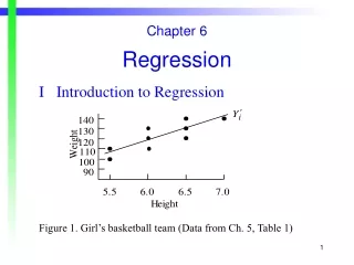
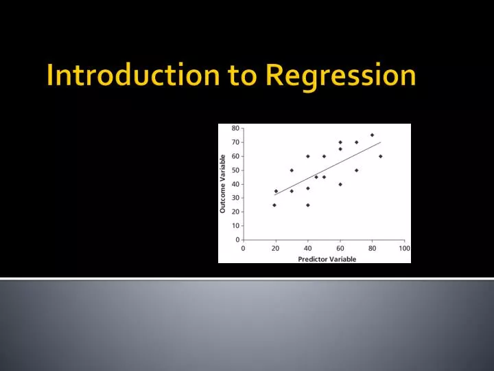
Introduction to Regression. Linear Regression. Ordinary Least Squares (OLS) Regression: A way of predicting an outcome as a linear function of other variables Simple Regression: one explanatory variable Multiple Regression : multiple explanatory variables (Next week’s topic). Outcome /

E N D
Linear Regression • Ordinary Least Squares (OLS) Regression: A way of predicting an outcome as a linear function of other variables • Simple Regression: one explanatory variable • Multiple Regression: multiple explanatory variables (Next week’s topic) Outcome / Dependent Variable Predictors / Independent Variables / Explanatory Variables
Importance of Regression • Basic OLS regression is considered by many to be the most widely used statistical techniques. • It was first studied in great depth by Sir Francis Galton, a 19th century naturalist, anthropologist and statistician. • Sort of a math-nerd version of Indiana Jones. • Began with his own studies of relative heights of fathers and sons. • Now used for basic analysis of experiments, hypothesis testing in various types of data, as well as predictive and machine-learning models.
The Idea behind Linear Regression • Fine a single line that best represents the relationship between X and Y. • Why a line? • The mean can be thought of as a model of a variable – the simplest one possible. • Aline is the next simplest way to model a variable. • Even in non-linear relationships, a line can be roughly approximate of an overall trend– which can still be very useful (especially when exploring data!) even if a line is not the most accurate way to describe the data.
Linear Regression as a Model • By using linear regression, we are assuming a linear relationship. This sounds simple and obvious enough, but it’s a big assumption. • Remember the most basic formula that comes up again and again in this course:
Linear Regression as a Model • So, in this case the term “model” can be replaced by the things that define a line. • We could just look at a scatterplot and kind of draw a line that more or less seems to fit the data, but this would be subjective. • So, linear regression is really just an objective way to find the best line to summarize data points. • Remember: we don’t necessarily even know if a single line is the best model to describe a given relationship. By conducting regression we effectively force a linear explanation onto our data.
Correlation versus Regression • Correlation is symmetric – it makes no assumption about whether one variable is dependent on the other. Correlation is only a measure of general linear association. • Regression attempts to model a single dependent variable as predicted by one or more explanatory variables. Assumes one-way link between X and Y.
Correlation versus Regression • Thus, correlation measures whether two variables share a linear relationship. Regression is a more precise description of a that relationship (e.g., the specific slope which is the change in Y given a change in X) • But, correlation is still a part of regression: the square of the correlation coefficient (R2) becomes an expression of how much of Y’s variance is explained by our model. • With regression, we now focus on the specifics of a linear relationship between two variables, X and Y.
Basic Interpretation Y = 98.4 – 0.761x • Our constant (y-intercept) is 98.4. • This means that the baseline school attendance with no child labor is 98.4%. • Our coefficient for X is -0.761. • So, if X = 10, we can calculate a predicted Y as 98.4 – (0.761* 10) = 90.8. Thus, each 10%increase in child laborcorresponds to a 7.61% decrease in school attendance.
The ‘ordinary least squares’ Solution (OLS) • When any line is fitted to a set of data, there will always be small differences between the exact data points and the line – these are called residuals • Residual for point i: • A good model for data should have small residuals – but how do we measure small? Observed value of y Predicted value of y
The Least Squares Solution (cont) • To choose a line of best fit, we square the residuals and take the sum • We then choose the line that minimizes the sum-squared residuals. • Why square residuals? • An extension of how the mean minimizes squared errors • Makes all residuals positive • Ensures – mathematically – that there is one and only one line of best fit. • Behind the scenes, the line of best fit can be computed algebraically – no iteration required. • Ordinary least squares is our method of estimation for a linear relationship. • Adapted from Myers, Gamst and Guarino 2006
Goodness of Fit • How do we know whether our linear model is a good representation of our data? • Residuals tell us something, but they’re not a good measure of overall fit. • The total sum-squared residual grows larger with more data points. • It also depends on the units we’re using.
The Coefficient of Determination (R2) • Instead, we can use r-squared (R2) to determine our model goodness of fit. • R is the same as r, the Pearson correlation coefficient. • R2 is the amount of variation in the outcome that can be explained by our model (which is just a single line). • Another way to compute R2is the model sum of squares divided by the total sum of squares. Or, the amount of variance in the outcome explained by the model, relative to how much variation we have to explain.
The Coefficient of Determination (R2) We can break down the total variation in our data into what our model explains, and what’s left over: • Total sum of squares (SST) is just the sum of squared differences between each data point and the mean, • Model (or Explained) sum of squares (SSM) is sum of the squared differences between each predicted data point and the mean, • This is the improvement in prediction that results from using the regression model rather than just the mean. • Residual sum of squares (SSR) is the sum of squared residuals • This is the unexplained variation. • In fact, SST = SSM + SSR • R2 = SSM / SST
The Coefficient of Determination (R2) • So, to recap: R2 is the amount of variance in the outcome explained by the model (our line), relative to how much total variation we have to explain (variation in our dependent variable). • The value for r-squared ranges from 0 to 1, and we can simply multiply the value by 100 to get a percentage interpretation. For example, an R2 = .25 means that our model can explain 25% of the variation in Y.
Assessing Statistical Significance yi= b0 + b1xi + ei. • Now that we know how to tell if our model is any good, how do we know if it is statistically significant or not? • Consider: What is the null hypothesis in a regression? • The null is that there is no linear relationship between X and Y. • Put in formal terms, the null hypothesis is b1 = 0. In other words, that our expectation for Yis not related to X. Or, that there is no slope. • Thus, a straight horizontal line means there is no linear relationship (sometimes this is counter-intuitive, but note that a horizontal line means that Y is the same for all values of X). No Linear Relationship Between X and Y
Assessing Statistical Significance • Since we just have one coefficient to test, we can use a t-test to see if it’s statistically different than zero. • We must use a t-distribution with n-2 degrees of freedom, since we are estimating two coefficients • If our t-test is significant, it means that b1 significantly different from zero and we become more confident that our predictor variable contributes to our ability to estimate values of our outcome variable.
Some of the key assumptions of linear regression • Our dependent variable is a quantitative, continuous variable. Usually this is a variable measured at the interval level. • We assume that the residuals (i.e., the error between the estimate and the actual values) are independent of each other (lack of autocorrelation). This is especially important in data that deals with time. • We assume that the residuals should be normally distributed. • The residuals should have the same variance at all levels of the predictor variable(s). This is homogeneity of variance, or homoscedasticity. • Also, we assume that a linear relationship is appropriate.
Regression Diagnostics • Autocorrelation: • Are the errors independent? • Heteroskedasticity: • Do the errors have a constant variance? • Linearity: • Is there a linear relationship between the dependent and independent variables? • Normality: • The error term should be normally distributed. (We can use the central limit theorem for large samples) • Outliers: • Do we have a few influential cases that may need to be dropped from the analysis? • Multicollinearity • If we have multiple predictor variables, are they too related to each other?
Problem: Autocorrelation • If the errors follow a distinct pattern (perhaps in only some places or along the regression line), then they are correlated with each other. They are not independent. • Autocorrelation is often called serial correlation as well. • Usually a problem to look for when the dependent variable deals with time. Example of Autocorrelated data. Errors from adjacent values are correlated with each other.
Checking for Autocorrelation • We can assess the independence of the errors by conducting a Durbin-Watson test, which can be conducted on a regression model. This is easy to run within R or any other general purpose statistical package. • If the Durbin-Watson test is statistically significant, then there is an issue with autocorrelation.
Problem: Heteroskedasticity • OLS regression assumes that the variance of the error term is constant. If the error does not have a constant variance, then it is heteroskedastic (literally, “different scatter”). http://www.unc.edu/~nielsen/soci709/m3/m3.htm
Heteroskedasticity (continued) • Consequences of Heteroskedasticity • OLS will not provide the estimate with the smallest variance. Where there is a lot of error, we become less confident in our line “of best fit”. • Why? Because OLS gives more ‘weight’ to the cases that might actually have the most error (distance) from the predicted line. Heteroskedasticity: uneven scatter
Heteroskedasticity (continued) • Detection: We have to look at the residuals (again, the difference between observed responses from the predicted responses) • Use a residual versus fitted (or predicted) values plot • We can also use a residuals versus predictor plot, which is a plot of the residuals versus one of the independent variables. • We should see an even band across the 0 point (the line), indicating that our error is roughly equal, like the visual example. • Note that for heteroskedasticity, we are just interested in whether the scatter is normal from left to right. Homoskedastic: (same width of scatter from left to right) Heteroskedastic: (different scatter from left to right).
Testing for Heteroskedasticity • If we are still concerned, we can run a test such as the Breusch-Pagan Test for Heteroskedasticity. It tests the null hypothesis that the error variances are all EQUAL, and the alternative hypothesis that there is some difference. • Thus, if out test for heteroskedasticity is statistically significant then we reject the null hypothesis and we do have a problem.
What to do about Heteroskedasticity? • Perhaps other variables better predict Y? • Could we transform Y without losing intuitive appeal? • If you are still interested in current independent variable “X”, you can conduct a robust regression which will adjust the model to account for heteroskedasticity. • Robust regression is helpful because it modifies the estimates for our standard errors and thus our t-tests for coefficients.
Problem : Checking Linearity • We should check to make sure that our data is actually linearly related. • We can examine the residuals versus predicted values plot (same as we use for heteroskedasticity). Example 1: Normal Example 2: Non-Linear (notice the bowed shape)
Fixing Linearity problems • One way to address a non-linear relationship is to transform the variable. • We can use transformations to shift a highly skewed distribution so that we can better fit a linear relationship between the independent and dependent variables.
Power Transformations • Helps to correct for skew and non-symmetric distributions. • Commonly used when the dependent variable in a regression is highly skewed. • Power transformations will not ‘fix’ distributions that are bimodal, uniform, etc. • Yq : reduces negative skew • Log Y or –(Y-q ): reduces positive skew
Interpreting a Power Transformation • Power transformations are not a magic wand– they only help you achieve symmetry and/or normality, but often symmetry is all you can hope to achieve. And, you still need to interpret the outcome! • We must reconvert our transformed Y back to normal units by using the inverse transformation: • Y* = Yq Y* 1/q = Y in original units • Y* = Loge Y eY* = Y in original units • So, when you calculate the predicted value from the regression equation, take the inverse transformation of the result: • We transformed Y with Y2. • Our regression is Y* = 3.2 X + 2.5 = 5.7 5.71/2 = 2.39 • Thus, when X =1, Y = 2.39 in its original units.
Problem: Checking Normality of Errors • If our error distribution is not normal, it will compromise our estimates for our coefficients and the calculation of statistical significance. • One of the best ways to test for the normality of distributed errors is to look at the normal probability plot of the residuals. If the distribution is normal, the points on the plot will fall close to the diagonal line. A bowed pattern or an S-shape pattern indicate typical problems (e.g., highly skewed errors or highly kurtotic residuals) Example normal probability plot of residuals Example from: http://www.r-tutor.com/elementary-statistics/simple-linear-regression/normal-probability-plot-residuals
Problem: Outliers • We already know that a few outliers can drastically shift our predicted line. • The solution is to look for cases that are far outside the norm: find the cases where we have very large residuals. As we will discuss later, we may also be interested in how much influence our outliers actually have on the model.
Problem: Issue with Multiple Independent Variables (Multicollinearity) • As we will discuss with multiple regression, we can also conduct regressions with many independent variables at the same time. • However, one of the other key issues we have to be aware of is “multicollinearity”, which is when independent variables are highly correlated with each other. • Since we are trying to predict a single line with different independent variables, high correlations between independent variables can lead to large errors in our model. • We will come back to this issue in the segments dedicated to multiple regression. At that point we will discuss how to test for multicollinearity and how to address it if it becomes a problem. • But… for now it is important to know the main diagnostics (heteroskedasticity, normality, and multicollinearity) that we typically use to check our regression assumptions.