Download
1 / 27
270 likes | 412 Vues
THE USE OF K-MEANS AND KOHONEN SELF ORGANIZING MAPS TO CLASSIFY COTTON BALES. J I Mwasiagi, Huang XiuBao, Wang XinHou & Chen Qing-Dong. Introduction.

E N D
THE USE OF K-MEANS AND KOHONEN SELF ORGANIZING MAPS TO CLASSIFY COTTON BALES J I Mwasiagi, Huang XiuBao, Wang XinHou & Chen Qing-Dong
Introduction • Cotton yarn characteristics such as length, micronaire, uniformity, short fiber index, spinning consistency, color and trash measurements can now be measured speedily using High Volume Instrument (HVI) • To properly utilize the high dimensional data obtained from HVI system, clustering techniques and other data analysis techniques can be used to describe the data
Kohonen Self Organizing Maps Kohonen Self Organizing Maps (SOM) whose architecture is given in figure 1, learn to recognize groups of similar input vectors in such a way that neurons physically close together in the neuron layer respond to similar input vectors
SOM • SOM learn both the distribution and topology of the input vectors they are trained on. The neurons in the layer of a SOM are arranged in physical positions according to given topology and distance functions • The quality of the SOM maps can be checked by using two factors: data representation accuracy and data set topology representation accuracy.
K-means clustering algorithm • Clustering algorithms attempt to organize unlabeled feature vectors into clusters or natural groupings • K means clustering algorithm constructs k (k fixed a priori) clusters for a given data set. • The K-means algorithm defines k centers one for each cluster and hence has k groups
K-means clustering algorithm • Place k points into the space represented by the objects that are being clustered. These points represent initial group centers. • Assign each object to the group whose center is closest. • When all objects have been assigned, recalculate the positions of the k centers. • Repeat the second and third steps until the centers no longer move. This produces a separation of the objects into groups from which the metric to be minimized can be calculated.
Quality of K-means clustering • Davies Bouldin (DB) index • Silhouette means
Statistical Techniques • Given a sample of data set for one attribute: • Descriptive measures such as measure of tendency and measure of dispersion • The results of the above analysis can be displayed using two dimensional graphs • For data with many attributes (High Dimensional data) • Principal components analysis technique
Materials and Methods Materials • HVI data obtained from Shanghai Inspection Center of Industrial Products and Materials (SICIPM) • The total data sample had 2421 cotton bales and 13 cotton 13 cotton lint characteristics were measured for each bale. • Data 2421x13 (High dimensional)
HVI Characteristics 13 cotton HVI characteristics: micronaire (Mic), maturity (Mat), length (Len), elongation (Elg), strength (Str), Short Fiber Index (Sfi), length uniformity (Unf), Spinning Consistency Index (Sci), reflectance (Rd), yellowness (+b), trash cent (Trc), trash area (Tra) and trash grade (Trg).
Methods • (i)Use SOM data visualization technique to get an idea of the nature of clustering within HVI data, • (ii) Partition the HVI data using K-means technique. The value of k should be obtained from (i) above, and • (iii) Check for data group compactness using other methods and techniques such as silhouette means, coefficient of variation and principal component analysis.
Methods (i) (i) Use SOM data visualization technique to get an idea of the nature of clustering within HVI data, (ii) (ii) Partition the HVI data using K-means technique. The value of k should be obtained from (i) above, and ( (iii) Check for data group compactness using other methods and techniques such as silhouette means, coefficient of variation and principal component analysis.
Result and Discussion Data Visualization • SOM reduced the 2421x13 data into 18x13 grids, with a quantization error of 1.879 and topographic error of 0.083. • The number of hits for each node of the SOM map is given in figure 2, which shows that there are multiple hits in 231 out of the 234 nodes of the visualization grids.
Data Clustering • Optimum clusters is 19 (fig. 3) • The means and the Coefficient of variation (CV) for the groups are given in Tables 1 and 2. • The CVs for the 2nd, 7th and 17th group are higher than that of the main group (MG) for some attributes. • 16 groups are properly partitioned
The Re-combined Subgroup (RSG) • 2nd, 7th and 17th groups re-combined and designated as RSG • Visualization and the hits for RSG is given in figure 4 • Level of grouping is very low with only five out of the 66 nodes having hits of more than 5, and about 44% of all the nodes have one (1) or zero hits.
Optimum clusters for RSG • The silhouette means for the RSG is given in figure 5. The optimum clustering is 3, which was the initial number of groups in RSG before re-combining. • Checking out the principal components of the attributes (Table 3), shows that 97. 87% of the variance is accounted for by the first two principal components.
Scatter plot for RSG • B and C are widely scattered and can be subdivided into two each-hence RSG has five groups • Still the five groups do not show a sense of compactness • RSG is just a collection of outliers
Conclusion • A cotton bale classification model has been proposed and used to classify 2421 cotton bales • The model reduced the 2421x13 HVI high dimensional data into 18x13 grids, with a quantization error of 1.879 and a topographic error of 0.083, and initially identified 19 groups in the data. • Three of the groups containing a total of 144 data failed the compactness test. The final classification of the 2421 cotton bales contains 16 groups of cotton bales having a total of 2277 bales and five sets of 144 bales containing outliers.
Thanks ! Q and A