Download
1 / 64
650 likes | 788 Vues
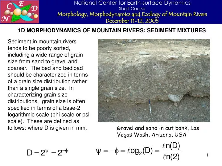
1D MORPHODYNAMICS OF MOUNTAIN RIVERS: SEDIMENT MIXTURES.

E N D
1D MORPHODYNAMICS OF MOUNTAIN RIVERS: SEDIMENT MIXTURES Sediment in mountain rivers tends to be poorly sorted, including a wide range of grain size from sand to gravel and coarser. The bed and bedload should be characterized in terms of a grain size distribution rather than a single grain size. In characterizing grain size distributions, grain size is often specified in terms of a base-2 logarithmic scale (phi scale or psi scale). These are defined as follows: where D is given in mm, Gravel and sand in cut bank, Las Vegas Wash, Arizona, USA
SEDIMENT GRAIN SIZE DISTRIBUTIONS The grain size distribution is characterized in terms of N+1 sizes Db,i such that ff,i denotes the mass fraction in the sample that is finer than size Db,i. In the example below N = 7. Note the use of a logarithmic scale for grain size.
SEDIMENT GRAIN SIZE DISTRIBUTIONS contd. In the grain size distribution of the last slide, the finest size (0.03125 mm) was such that 2 percent, not 0 percent was finer. If the finest size does not correspond to 0 percent content, or the coarsest size to 100 percent content, it is often useful to use linear extrapolation on the psi scale to determine the missing values. Note that the addition of the extra point has increased N from 7 to 8 (there are N+1 points).
SEDIMENT GRAIN SIZE DISTRIBUTIONS contd. The grain size distribution after extrapolation is shown below.
CHARACTERISTIC SIZES BASED ON PERCENT FINER Dx is size such that x percent of the sample is finer than Dx Examples: D50 = median size D90 ~ roughness height To find Dx (e.g. D50) find i such that Then interpolate for x and back-calculate Dx in mm
STATISTICAL CHARACTERISTICS OF SIZE DISTRIBUTION N+1 bounds defines N grain size ranges. The ith grain size range is defined by (Db,i, Db,i+1) and (ff,i, ff,i+1) i (Di) = characteristic size of ith grain size range fi = fraction of sample in ith grain size range
STATISTICAL CHARACTERISTICS OF SIZE DISTRIBUTION contd. = mean grain size on psi scale = standard deviation on psi scale Dg= geometric mean size g = geometric standard deviation ( 1) Sediment is well sorted if g < 1.6 Dg = 0.273 mm, g = 2.17
GRAIN SIZE DISTRIBUTION CALCULATOR Workbook RTe-bookGSDCalculator.xls computes the statistics of a grain size distribution input by the user, including Dg, g, and Dx where x is a specified number between 0 and 100 (e.g. the median size D50 for x = 50). It uses code in VBA (macros) to perform the calculations. You will not be able to use macros if the security level in Excel is set to “High”. To set the security level to a value that allows you to use macros, first open Excel. Then click “Tools”, “Macro”, “Security…” and then in “Security Level” check “Medium”. This will allow you to use macros.
GRAIN SIZE DISTRIBUTION CALCULATOR contd. When you open the workbook RTe-bookGSDCalculator.xls, click “Enable Macros”. The GUI is contained in the worksheet “Calculator”. Now to access the code, from any worksheet in the workbook click “Tools”, “Macro”, “Visual Basic Editor”. In the “Project” window to the left you will see the line “VBA Project (FDe-bookGSDCalculator.xls)”. Underneath this you will see “Module1”. Double-click on “Module1” to see the code in the “Code” window to the right. These actions allow you to see the code, but not necessarily to understand it. In order to understand this course, you need to learn how to program in VBA. Please work through the tutorial contained in the workbook RTe-bookIntroVBA.xls. It is not very difficult! All the input are specified in the worksheet “Calculator”. First input the number of pairs npp of grain sizes and percents finer (npp = N+1 in the notation of the previous slides) and click the appropriate button to set up a table for inputting each pair (grain size in mm, percent finer) in order of ascending size. Once this data is input, click the appropriate button to compute Dg and g. To calculate any size Dx where x denotes the percent finer, input x into the indicated box and click the appropriate button. To calculate Dx for a different value of x, just put in the new value and click the button again.
GRAIN SIZE DISTRIBUTION CALCULATOR contd. This is what the GUI in worksheet “Calculator” looks like.
GRAIN SIZE DISTRIBUTION CALCULATOR contd. If the finest size in the grain size distribution you input does not correspond to 0 percent finer, or if the coarsest size does not correspond to 100 percent finer, the code will extrapolate for these missing sizes and modify the grain size distribution accordingly. The units of the code are “Sub”s (subroutines). An example is given below. Sub fraction(xpf, xp) 'computes fractions from % finer Dim jj As Integer For jj = 1 To np xp(jj) = (xpf(jj) - xpf(jj + 1)) / 100 Next jj End Sub In this Sub, xpf denotes a dummy array containing the percents finer, and xp denotes a dummy array containing the fractions in each grain size range. The Sub computes the fractions from the percents finer. Suppose in another Sub you know the percents finer Ff(i), I = 1..npp and wish to compute the fraction in each grain size range F(i), i = 1..np (where np = npp – 1). The calculation is performed by the statement fraction Ff, f
WHY CHARACTERIZE GRAIN SIZE DISTRIBUTIONS IN TERMS OF A LOGARITHMIC GRAIN SIZE? Consider a sediment sample that is half sand, half gravel (here loosely interpreted as material coarser than 2 mm), ranging uniformly from 0.0625 mm to 64 mm. Plotted with a logarithmic grain size scale, the sample is correctly seen to be half sand, half gravel. Plotted using a linear grain size scale, all the information about the sand half of the sample is squeezed into a tiny zone on the left-hand side of the diagram. Logarithmic scale for grain size Linear scale for grain size
UNIMODAL AND BIMODAL GRAIN SIZE DISTRIBUTIONS The fractions fi(i) represent a discretized version of the continuous function f(), f denoting the mass fraction of a sample that is finer than size . The probability density pf of size is thus given as p = df/d. The example to the left corresponds to a Gaussian (normal) distribution with = -1 (Dg = 0.5 mm) and = 0.8 (g = 1.74): The grain size distribution is called unimodel because the function p() has a single mode, or peak. The following approximations are valid for a Gaussian distribution:
UNIMODAL AND BIMODAL GRAIN SIZE DISTRIBUTIONS contd. A sand-bed river has a characteristic size of bed surface sediment (D50 or Dg) that is in the sand range. A gravel-bed riverhas a characteristic bed size that is in the range of gravel or coarser material. The grain size distributions of most sand-bed streams are unimodal, and can often be approximated with a Gaussian function. Many gravel-bed river, however, show bimodalgrain size distributions, as shown to the upper right. Such streams show a sand mode and a gravel mode, often with a paucity of sediment in the pea-gravel size (2 ~ 8 mm). Plateau Gravel mode Sand mode A bimodal (multimodal) distribution can be recognized in a plot of f versus in terms of a plateau (multiple plateaus) where f does not increase strongly with .
UNIMODAL AND BIMODAL GRAIN SIZE DISTRIBUTIONS contd. The grain size distributions to the left are all from 177 samples from various river reaches in Alberta, Canada (Shaw and Kellerhals, 1982). The samples from sand-bed reaches are all unimodal. The great majority of the samples from gravel-bed reaches show varying degrees of bimodality. Note: geographers often reverse the direction of the grain size scale, as seen to the left. Figure adapted from Shaw and Kellerhals (1982)
VERTICAL SORTING OF SEDIMENT Gravel-bed rivers such as the River Wharfe often display a coarse surface armor or pavement. Sand-bed streams with dunes such as the one modeled experimentally below often place their coarsest sediment in a layer corresponding to the base of the dunes. River Wharfe, U.K. Image courtesy D. Powell. Sediment sorting in a laboratory flume. Image courtesy A. Blom.
EXNER EQUATION OF CONSERVATION OF BED SEDIMENT FOR SIZE MIXTURES MOVING AS BEDLOAD fi'(z', x, t) = fractions at elevation z' in ith grain size range above datum in bed [1]. Note that over all N grain size ranges: qbi(x, t) = volume bedload transport rate of sediment in the ith grain size range [L2/T] Or thus:
ACTIVE LAYER CONCEPT The active, exchange or surface layer approximation (Hirano, 1972): Sediment grains in active layer extending from - La < z’ < have a constant, finite probability per unit time of being entrained into bedload. Sediment grains below the active layer have zero probability of entrainment.
REDUCTION OF SEDIMENT CONSERVATION RELATION USING THE ACTIVE LAYER CONCEPT Fractions Fi in the active layer have no vertical structure. Fractions fi in the substrate do not vary in time. Thus where the interfacial exchange fractions fIi defined as describe how sediment is exchanged between the active, or surface layer and the substrate as the bed aggrades or degrades.
REDUCTION OF SEDIMENT CONSERVATION RELATION USING THE ACTIVE LAYER CONCEPT contd. Between and it is found that (Parker, 1991).
REDUCTION contd. The total bedload transport rate summed over all grain sizes qbT and the fraction pbi of bedload in the ith grain size range can be defined as The conservation relation can thus also be written as Summing over all grain sizes, the following equation describing the evolution of bed elevation is obtained: Between the above two relations, the following equation describing the evolution of the grain size distribution of the active layer is obtained:
EXCHANGE FRACTIONS where 0 1 (Hoey and Ferguson, 1994; Toro-Escobar et al., 1996). In the above relations Fi, pbi and fi denote fractions in the surface layer, bedload and substrate, respectively. That is: The substrate is mined as the bed degrades. A mixture of surface and bedload material is transferred to the substrate as the bed aggrades, making stratigraphy. Stratigraphy (vertical variation of the grain size distribution of the substrate) needs to be stored in memory as bed aggrades in order to compute subsequent degradation.
ALTERNATIVE DIMENSIONLESS BEDLOAD TRANSPORT The generalized bedload transport relation of the type of Meyer-Peter and Müller (1948) was written in the form: where Recalling that b = u*2, the relation can be written in the alternative form where (Parker et al., 1982). The form W* versus * is often used as the basis for generalizing to sediment mixtures.
SURFACE-BASED BEDLOAD TRANSPORT FORMULATION FOR MIXTURES Consider the bedload transport of a mixture of sizes. The thickness La of the active (surface) layer of the bed with which bedload particles exchange is given by as where Ds90 is the size in the surface (active) layer such that 90 percent of the material is finer, and na is an order-one dimensionless constant (in the range 1 ~ 2). Divide the bed material into N grain size ranges, each with characteristic size Di, and let Fi denote the fraction of material in the surface (active) layer in the ith size range. The volume bedload transport rate per unit width of sediment in the ith grain size range is denoted as qbi. The total volume bedload transport rate per unit width is denoted as qbT, and the fraction of bedload in the ith grain size range is pbi, where Now in analogy to *, q* and W*, define the dimensionless grain size specific Shields number i*, grain size specific Einstein number qi* and dimensionless grain size specific bedload transport rate Wi* as
SURFACE-BASED BEDLOAD TRANSPORT FORMULATION contd. It is now assumed that a functional relation exists between qi* (Wi*) and i*, so that The bedload transport rate of sediment in the ith grain size range is thus given as According to this formulation, if the grain size range is not represented in the surface (active) layer, it will not be represented in the bedload transport.
BEDLOAD RELATION FOR MIXTURES DUE TO PARKER (1990) This relation is appropriate only for the computation of gravel bedload transport rates in gravel-bed streams. In computing Wi*, Fi must be renormalized so that the sand is removed, and the remaining gravel fractions sum to unity, Fi = 1. The method is based on surface geometric size Dsg and surface arithmetic standard deviation s on the scale, both computed from the renormalized fractions Fi. In the above O and O are set functions of sgospecified in the next slide.
BEDLOAD RELATION FOR MIXTURES DUE TO PARKER (1990) contd. o o It is not necessary to use the above chart. The calculations can be performed using the Visual Basic programs in RTe-bookAcronym1.xls
BEDLOAD RELATION FOR MIXTURES DUE TO WILCOCK AND CROWE (2003) The sand is not excluded in the fractions Fi used to compute Wi*. The method is based on the surface geometric mean size Dsg and fraction sand in the surface layer Fs.
AGGRADATION AND DEGRADATION OF RIVERS TRANSPORTING GRAVEL MIXTURES Results of a flood in the gravel-bed Salmon River, Idaho. Photo by author
MODELING AGGRADATION AND DEGRADATION IN GRAVEL-BED RIVERS CARRYING SEDIMENT MIXTURES Gravel-bed rivers tend to be steep enough to allow the use of the normal (steady, uniform) flow approximation. Here this analysis is applied using a Manning-Strickler formulation such that roughness height ks is given as where Ds90 is the size of the surface material such that 90% is finer and nk is an order-one dimensionless number (1.5 ~ 3; the work of Kamphuis, 1974 suggests a value of 2). No attempt is made here to decompose bed resistance into skin friction and form drag. The reach is divided into M intervals bounded by M + 1 nodes. In addition, sediment is introduced at a ghost node at the upstream end. Since the index “i” has been used for grain size ranges, the index “k” is used here for spatial nodes.
COMPUTATION OF BED SLOPE AND BOUNDARY SHEAR STRESS At any given time t in the calculation, the bed elevation k and surface fractions Fi,k must be known at every node k. The roughness height ks,k and thickness of the surface layer La,k are computed from the relations where nk and na are specified order-one dimensionless constants. (Beware: in the equation for roughness height the “k” in nk is not an index for spatial node.) Using the normal flow approximation, the boundary shear stress b,k at the kth node is given from Chapter 5 as where u,k denotes the shear velocity and bed slope Sk is computed as Bed slope need not be computed at k = M + 1, where bed elevation is specified as a boundary condition.
COMPUTATION OF BEDLOAD TRANSPORT Once Fi,k and b,k are known, the bedload transport rates qbi, and thus qbT and pi can be computed at any node. An example is given here in terms of the Wilcock-Crowe (2003) formulation. The surface geometric mean size Dsg,k is calculated at every node as where i = ln2(Di). The Shields number and shear velocity based on the surface geometric mean size are then given as The same fractions Fi,k allow the computation of the fraction sand Fs,k in the surface layer at node k. This parameter is needed in the formulation of Wilcock and Crowe (2003).
COMPUTATION OF BEDLOAD TRANSPORT contd. It follows that the volume bedload transport rate per unit width in the ith grain size range is given as where in the case of the relation of Wilcock and Crowe (2003),
MODELING AGGRADATION AND DEGRADATION IN GRAVEL-BED RIVERS CARRYING SEDIMENT MIXTURES contd. The discretized versions of the Exner relations are: where fIi,k is evaluated from a relation of the type given in Slide 4: In the above relation fs,i,int,k denotes the fractions of the substrate just below the surface layer at node k and is a user-specified parameter between 0 and 1.
MODELING AGGRADATION AND DEGRADATION IN GRAVEL-BED RIVERS CARRYING SEDIMENT MIXTURES contd. The spatial derivatives of the sediment transport rates are computed as where au is a upwinding coefficient equal to 0.5 for a central difference scheme. When k = 1, the node k – 1 refers to the ghost node, where qbi, and thus qbT and pi are specified as feed parameters. The term La,k/t t is not a particularly important one, and can be approximated as where La,k,old is the value of La,k from the previous time step. In the case of the first time step, La,k,old may be set equal to 0.
BOUNDARY CONDITIONS, INITIAL CONDITIONS AND FLOW OF THE COMPUTATION • The boundary conditions are • Specified values of qb,i (and thus qbT and pbi) at the upstream ghost node; • Specified bed elevation at node k = M+1. • The initial conditions are • Specified initial bed elevations at every node (here simplified to a specified initial bed slope Sfbl; • Specified surface and substrate grain size distributions Fi and fs,i at every node (here taken to be the same at every node). • At any given time fractions Fi and elevation are known at every node. The values Fi are used to compute Ds90 Dsg, Ds50, ks, La and other parameters (e.g. Fs) at every node. The values of are used to compute slopes S and combined with the computed values of ks to determine the shear stress b at every node except M+1, where the information is not needed. The resulting parameters are used to compute qbi, qbT and pbi at all nodes except M+1. The Exner relations are then solved to determine bed elevations and surface fractions Fi at all nodes. At node M+1 only the change in grain size distribution is evaluated.
INTRODUCTION TO RTe-bookAgDegNormGravMixPW.xls The workbook is a descendant of the PASCAL code ACRONYM3 of Parker (1990a,b). It allows the user to choose from two surface-based bedload transport formulations; those of Parker (1990) and Wilcock and Crowe (2003). In the relation of Parker (1990) the surface grain size distributions need to be renormalized to exclude sand before specification as input to the program. This step is neither necessary nor desirable in the case of the relation of Wilcock and Crowe (2003), where the sand plays an important role in mediating the gravel bedload transport. The basic input parameters are the water discharge per unit width qw, flood intermittency If, gravel input rate during floods qbTf, reach length L, initial bed slope SfbI, number of spatial intervals M, time step t, fractions pbf,i of the gravel feed, fractions FI,i of the initial surface layer (assumed the same at every node) and fractions fsI,I of the substrate (assumed to be uniform in the vertical and the same at every node). The parameters Mprint and Mtoprint control output. Auxiliary parameters include nk for roughness height, na for active layer thickness, r of the Manning-Strickler relation, submerged specific gravity R of the sediment, bed porosity p, upwinding coefficient au and interfacial transfer coefficient .
INTRODUCTION TO RTe-bookAgDegNormGravMixPW.xls contd. One interesting problem of sediment mixtures is when the river first aggrades, creating its own substrate with a vertical structure in the process, and then degrades into it. The code in the workbook is not set up to handle this. The necessary extension is trivial in theory but tedious in practice; the vertical structure of the newly-created substrate must be stored in memory as the calculation proceeds. A gravel-bed reach of the Las Vegas Wash, USA, where the river is degrading into its own deposits. Some calculations with the code follow.
CALCULATIONS WITH RTe-bookAgDegNormGravMixPW.xls The calculations are performed with the Parker (1990) bedload transport relation. The grain size distributions of the feed sediment, initial surface sediment and substrate sediment are all taken to be identical, as given below. Note that sand has been removed from the grain size distributions.
CALCULATIONS WITH RTe-bookAgDegNormGravMixPW.xls contd. A case is chosen for which the bed must aggrade from a very low slope. Calculations are performed for 60 years, 600 years and 6000 years in order to study the evolution of the profile. The software produces graphical output for the time development of the long profiles of a) bed elevation , b) surface geometric mean size Dsg and c) volume gravel bedload transport rate per unit width qbT.
Parker relation After 60 years
Parker relation After 60 years
Downstream variation of qbT/qbTf, where qbT = Bedload Transport Rate and qbTf = Upstream Bedload Feed Rate Parker relation After 60 years qbT/qbTf
Parker relation After 600 years
Parker relation After 600 years
Downstream variation of qbT/qbTf, where qbT = Bedload Transport Rate and qbTf = Upstream Bedload Feed Rate Parker relation After 600 years qbT/qbTf
Parker relation After 6000 years
Parker relation After 6000 years
Downstream variation of qbT/qbTf, where qbT = Bedload Transport Rate and qbTf = Upstream Bedload Feed Rate Parker relation After 6000 years qbT/qbTf