Chap 10. Sensitivity Analysis

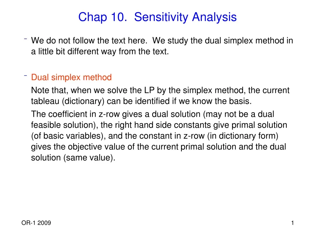
1. Chap 10. Sensitivity Analysis • We do not follow the text here. We study the dual simplex method in a little bit different way from the text. • Dual simplex method Note that, when we solve the LP by the simplex method, the current tableau (dictionary) can be identified if we know the basis. The coefficient in z-row gives a dual solution (may not be a dual feasible solution), the right hand side constants give primal solution (of basic variables), and the constant in z-row (in dictionary form) gives the objective value of the current primal solution and the dual solution (same value).

2. Dual simplex method is a variant of the simplex method which tries to find a basis which satisfies the primal feasibilitywhile the dual feasibility (optimality condition) is always maintained (i.e. the coefficients in z-row are all nonpositive) • Useful when we can easily find a dual feasible but primal infeasible basis. (e.g. We solved a problem to optimality, hence have found an optimal basis. But we want to solve the problem again with the right hand sides changed, and/or add a constraint which is violated by the current optimal solution. )

3. Assume that we have LP in the form max c’x Ax = b x  0 Its dual is min y’b y’A  c’ y unrestricted Optimality condition for simplex method to solve the primal problem is cj – y’Aj  0, j N. It is the dual feasibility condition.

4. Algorithm • Given a simplex tableau (with basis B) with and 1. Find row l with xB(l)< 0. Let vibe the l-th component of the columns B-1Ai , i  N. 2. For i with vi< 0, find nonbasic j such that 3. Perform pivot with variable xjentering and xB(l) leaving the basis.

5. example given in tableau form Current basis is {x4, x5} leaving basic variable is x5, entering nonbasic variable is determined by min{(-6)/(-2), (-10)/(-3)} = 3 Hence x2 is entering. After pivot, we get Note that, after the pivot, the objective value decreases ( 0  (-3) ) (dual is a minimization problem). Dual feasibility maintained.

6. Remarks • Note that we first choose the leaving basic variable, and then the entering nonbasic variable. • If all coefficients in row l are nonnegative, it implies that the LP is infeasible. ( Suppose we have 2, 3 in place of –2, -3 in our example. So the last row is , which cannot be satisfied by any nonnegative variables x.) Then the dual problem is unbounded since primal is infeasible and dual has a feasible solution.

7. Changes in the Data • Want to identify the range of data change which does not change the optimal basis. • Current basis B is said to be an optimal basis if B-1b  0 and (cN’ – cB’B-1N)  0. • Consider an example. Optimal tableau is • max 5x1 + x2 - 12x3 • s.t. 3x1 + 2x2 + x3 = 10 • 5x1 + 3x2 + x4 = 16 • x1, … , x4 0 B-1

8. Changes in the rhs b: Suppose the rhs bi is changed to bi + . Then current basis is still optimal basis as long as B-1(b + ei ) = B-1b +  B-1ei  0. (Note that B-1ei is i-th column of B-1 ) (ei is i-th unit vector). ex) Suppose b1  10 +  Then Note that the interpretation of optimal dual variable value y1 as marginal cost of the first resource applies for this range of  (recall Theorem 5.5).

9. Changes in the objective coefficient c: (1) cj cj +  for nonbasic variable xj If we perform the same elementary row operations to the changed data, we will have cj cj +  at the current optimal tableau. Current basis remains optimal as long as cj +   0. ex) c3 -12 + , then c3 becomes -2 +  ( 0)    2 (2) cj cj +  for basic variable xj (assume xj is k-th basic var) Using the same logic as above, we will have cj 0 +  at the current optimal tableau. We may perform elementary row operation to make the reduced cost of xj equal to 0. It corresponds to computing the dual vector y again using y’ = (cB’ + ek’)B-1. Then the reduced costs of nonbasic variables change. Check the range of  which makes the reduced costs  0.

10. Ex) Suppose c1 5 + . Then the optimal tableau changes to Perform elementary row operation to make c1 to 0. From -2 + 3  0, -7 - 2  0, we obtain -7/2    2/3.