Download
1 / 28
280 likes | 289 Vues
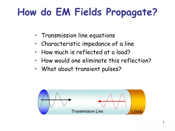
This text provides an overview of how electromagnetic fields propagate and interact in transmission lines, electrostatics, and magnetostatics. It covers topics such as transmission line equations, characteristic impedance, reflection at loads, elimination of reflections, interaction of static charges, and Maxwell's equations.

E N D
Transmission Line LOAD How do EM Fields Propagate? • Transmission line equations • Characteristic impedance of a line • How much is reflected at a load? • How would one eliminate this reflection? • What about transient pulses?
+ + + + + + + + + How do static charges interact? (Electrostatics) F2 F1 r Coulomb’s Law Force q1q2/r2 q2 q1 Gauss’s Law Flux q1 + q2 + .. Interaction in materials (Polarization)
E = lim F/q q 0 Vector Fields(A “disturbance in the force”) q
Non-negligible q Vector Fields(A disturbance in the force)
I1 i21 I dl2 i12 R I2 dl1 r H How do magnetic fields interact?(Magnetostatics) Biot-Savart’s Law Current magnetic field H ~ I/r Another current senses it Force ~ i2 x H
I r H Time variation couples E and H Ampere’s Law Varying E produces H Faraday’s Law Varying H produces E
E E E E H H H Varying E produces H produces E produces H .. Faraday’s Law Ampere’s Law Coulomb/Gauss’ Law Gauss’ law for magnets Electrodynamics Maxwell’s Eqns.
Faraday’s Law Ampere’s Law Coulomb/Gauss’ Law Gauss’ law for magnets Electrodynamics Don’t worry about memorizing these yet – We will come back to these later. But meanwhile, let’s try to understand them qualitatively....
I r H Deciphering Maxwell’s equations Q Magnetic fields curl but don’t diverge Electric fields diverge but don’t curl
I r H Deciphering Maxwell’s equations Q Magnetic fields curl but don’t diverge (they loop on themselves since there are no magnetic poles) Electric fields diverge but don’t curl (they start and end on charges or ‘poles’)
I r H We thus have Maxwell’s equations in theirsimplest form (for static sources, in vacuum) Q Curl(H) I Div(H) = 0 Div(E) Q Curl(E) = 0 We will define Div and Curl precisely later on. For now, think of them as the number of diverging and curling lines respectively
E • E • E • E • H • H • H Note how E and H equations are independent of each other !! This is true for static sources For dynamic sources (time-dependent currents), you also get dH/dt terms for the E equations and dE/dt terms for the H equations, which couple them. • Varying E produces H produces E produces H .. We thus have Maxwell’s equations in theirsimplest form (for static sources, in vacuum) Curl(H) I Div(H) = 0 Div(E) Q Curl(E) = 0
Consequences of Maxwell’s equations Waves Radiation
Traveling Waves Direction of propagation Wavefront f+(x-vt)
f+(x) t=0 x0=vt0 f+(x-x0) x1=vt1 t=t0 f+(x-x1) t=t1 xt=vt f+(x-xt) t x1 xt x0 Wave propagation f+(x-vt)
Sinusoid ASin(x-vt) For propagation direction, only relative sign between x and t matters
Sinusoid ASin(x+vt) For propagation direction, only relative sign between x and t matters
Decaying Sinusoid Ae-axSin(x-vt) Propagation in a lossy medium
Electromagnetic Spectrum Application determined by wavelength http://lectureonline.cl.msu.edu/~mmp/applist/Spectrum/s.htm
Periodicity/Wavelength y = Asin[2p(t/T – x/l)] Frequency f = 1/T Angular Frequency w=2pf = 2p/T Wavenumber n = 1/l Wavevector/Prop const • = 2p/l y = Asin[2pt/T] y = Asin[2px/l] ~ y = Asin[wt-bx]
ejq = cos(q) + jsin(q) Euler’s Formula Profound!! Connects algebra with trig! Converts PDEs into algebraic equations!! d/dq[ej(aq)] = a[ej(aq)] ∫dqej(aq) = ej(aq)/a Trig identities become algebraic identities!! ejq1.ejq2 = ej(q1+q2) Complex #s, Phasors
ejq = cos(q) + jsin(q) • e-jq = cos(q) - jsin(q) • cos(q) = [ejq+e-jq]/2 • sin(q) = [ejq-e-jq]/2j sin(A+B) = [ej(A+B)-e-j(A+B)]/2j = [ejA.ejB-e-jA.e-jB]/2j = ([cosA+jsinA][cosB+jsinB]-[cosA-jsinA][cosB-jsinB])/2j = ([cosAcosB+jsinAcosB+jcosAsinB-sinAsinB] -[cosAcosB-jsinAcosB-jcosAsinB+sinAsinB])/2j = sinAcosB-cosAsinB
ejq = cos(q) + jsin(q) z = |z|ejq = |z|q z* = |z|e-jq = |z|-q z1z2= (|z1|ejq1)(|z2|ejq2) = |z1||z2|(q1 + q2) Complex #s, Phasors • zn=|z|nnq • z1/2=|z|1/2q/2 (q unknown upto2pm) • z-1=|z|-1-q • z1/z2= (|z1|ejq1)/(|z2|ejq2) = |z1|/|z2|(q1 - q2)
z = a + jb z* = a – jb Complex Conjugate zz* = a2 + b2 |z| = zz* = (a2+b2) Magnitude/Norm/Amplitude 1/z = z*/|z|2 = (a-jb)/(a2+b2) Rationalizing z=|z|ejq= |z|(cosq + jsinq) Phasor notation |z|cosq = a, |z|sinq = b Components |z| = (a2+b2), q = tan-1(b/a) Complex #s
Phasor examples LC PhasorRC PhasorRL PhasorRLC Circuit
R L coswt+jsinwt V0cos(wt) ~ ~ i =Re(iejwt) ~ V = Re(Vejwt) ~ ~ [R + jLw] i = V ~ ~ ~ i = V/[R+jLw] = V[R-jLw]/{R2+L2w2} cos(wt) = Re[ejwt] sin(wt) = Im[ejwt] = Re[-jejwt] = Re[ej(wt-p/2)] Ri + Ldi/dt = V0cos(wt) i = Re(V0ejwt[R-jLw]/{R2+L2w2}) = V0(Rcoswt+Lwsinwt)/{R2+L2w2}
R L V0cos(wt) ~ ~ i =Re(iejwt) ~ V = Re(Vejwt) ~ ~ [R + jLw] i = V ZR ZL(w) Impedance Ri + Ldi/dt = V0cos(wt) ZC(w) = 1/jwC = -j/wC Try an LC circuit !!