Download
1 / 62
650 likes | 847 Vues
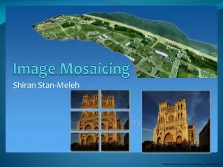
Image Mosaicing. Shiran Stan-Meleh. *http ://www.ptgui.com/info/image_stitching.html. Why do we need it?. Satellite Images. 360 View. Panorama. Compact Camera FOV = 50 x 35° Human FOV = 200 x 135° Panoramic Mosaic = 360 x 180°. How do we do it?. 2 methods.

E N D
Image Mosaicing Shiran Stan-Meleh *http://www.ptgui.com/info/image_stitching.html
Why do we need it? Satellite Images 360 View Panorama • Compact Camera FOV = 50 x 35° • Human FOV = 200 x 135° • Panoramic Mosaic = 360 x 180°
How do we do it? 2 methods • Direct (appearance-based) • Search for alignment where most pixels agree • Feature-based • Find a few matching features in both images • compute transformation *Copied from Hagit Hel-Or ppt
How do we do it? Direct (appearance-based) methods Manually… *http://www.marymount.fr/uploads/galleries/gallery402/images/002_matisse_project_gluing.jpg
How do we do it? Direct (appearance-based) methods • Define an error metric to compare the imagesEx: Sum of squared differences (SSD). • Define a search technique (simplest: full search) Pros: • Simple algorithm, can work on complicated transformation • Good for matching sequential frames in a video Cons: • Need to manually estimate parameters • Can be very slow
How do we do it? Feature based methods • Harris Corner detection - C. Harris &M. Stephens (1988) • SIFT - David Lowe (1999) • PCA-SIFT - Y. Ke & R. Sukthankar (2004) • SURF - Bay & Tuytelaars (2006) • GLOH - Mikolajczyk & Schmid (2005) • HOG - Dalal & Triggs (2005)
Agenda We will concentrate on feature based methods using SIFT for features extraction and RANSAC for features matching and transformation estimation
Some Background SIFT and RANSAC
What is SIFT? Scale Invariant Features Transform From Wiki: “an algorithm in computer vision to detect and describe local features in images. The algorithm was published by David Lowe in 1999”
Applications • Object recognition • Robotic mapping and navigation • Image stitching • 3D modeling • Gesture recognition • Video tracking • Individual identification of wildlife • Match moving
Basic Steps • Scale Space extrema detection • Construct Scale Space • Take Difference of Gaussians • Locate DoG Extrema • Keypoint localization • Orientation assignment • Build Keypoint Descriptors *http://www.csie.ntu.edu.tw/~cyy/courses/vfx/05spring/lectures/handouts/lec04_feature.pdf
1a. Construct Scale Space Motivation: Real-world objects are composed of different structures at different scales First Octave Explanation: representing an image at different scales at different blurred levels Second Octave *copied from Hagit Hel-Or ppt
1b. Take Difference of Gaussians • Experimentally, Maxima of Laplacian-of-Gaussian (LoG: ) gives best notion of scale: • But it’s extremely costly so instead we use DoG: *Distinctive Image Features from Scale-Invariant Keypoints David G. Lowe *Mikolajczyk 2002
1c. Locate DoG Extrema • Find all Extrema, that is minimum or maximum in 3x3x3 neighborhood: *Distinctive Image Features from Scale-Invariant Keypoints David G. Lowe
Basic Steps • Scale Space extrema detection • Keypoint localization • Sub Pixel Locate Potential Feature Points • Filter Edge and Low Contrast Responses • Orientation assignment • Build Keypoint Descriptors *http://www.csie.ntu.edu.tw/~cyy/courses/vfx/05spring/lectures/handouts/lec04_feature.pdf
2a. Sub Pixel Locate Potential Feature Points • Problem: • Solution:Take Taylor series expansion:Differentiate and set to 0 to get location in terms of : *http://www.inf.fu-berlin.de/lehre/SS09/CV/uebungen/uebung09/SIFT.pdf
2b. Filter Edge and Low Contrast Responses • Remove low contrast points (sensitive to noise): • Remove keypoints with strong edge response in only one direction (how?): *http://www.inf.fu-berlin.de/lehre/SS09/CV/uebungen/uebung09/SIFT.pdf
2b. Filter Edge and Low Contrast Responses • By using Hessian Matrix: • Eigenvalues of Hessian matrix are proportional to principal curvatures • Use Trace and Determinant: • R=10, only 20 floating points operations per Keypoint
“Picture worth a 1000 keypoints” • Original image • Low contrast removed (729) • Initial features (832) • Low curvature removed (536) *Distinctive Image Features from Scale-Invariant Keypoints David G. Lowe
Basic Steps • Scale Space extrema detection • Keypoint localization • Orientation assignment • Build Keypoint Descriptors Low contrast removed Low curvature removed *http://www.csie.ntu.edu.tw/~cyy/courses/vfx/05spring/lectures/handouts/lec04_feature.pdf
3. Orientation assignment • Compute gradient magnitude and orientation for each SIFT point : • Create gradient histogram weighted by Gaussian window with = 1.5* and use parabola fit to interpolate more accurate location of peak. *http://www.inf.fu-berlin.de/lehre/SS09/CV/uebungen/uebung09/SIFT.pdf
Basic Steps • Scale Space extrema detection • Keypoint localization • Orientation assignment • Build Keypoint Descriptors *http://www.csie.ntu.edu.tw/~cyy/courses/vfx/05spring/lectures/handouts/lec04_feature.pdf
4. Build Keypoint Descriptors • 4x4 Gradient windows relative to keypoint orientation • Histogram of 4x4 samples per window in 8 directions • Gaussian weighting around center( is 0.5 times that of the scale of a keypoint) • 4x4x8 = 128 dimensional feature vector • Normalize to remove contrast • perform threshold at 0.2 and normalize again *Image from: Jonas Hurrelmann
Live DemoAnd next…RANSAC *http://habrahabr.ru/post/106302/
What is RANSAC? RANdom SAmple Consensus • first published by Fischler and Bolles at SRI International in 1981 • From Wiki: • An iterative method to estimate parameters of a mathematical model from a set of observed data which contains outliers • Non Deterministic • Outputs a “reasonable” result with certain probability
What is RANSAC? A data set with many outliers for which a line has to be fitted Fitted line with RANSACoutliers have no influence on the result *http://en.wikipedia.org/wiki/RANSAC
RANSAC Input & Output The procedure is iterated k times, for each iteration: • Input • Set of observed data values • Parameterized model which can explain or be fitted to the observations • Some confidence parameters • Output • Best model - model parameters which best fit the data (or nil if no good model is found) • Best consensus set - data points from which this model has been estimated • Best error - the error of this model relative to the data
Basic Steps • Select a random subset of the original data called hypothetical inliers • Fill free parameters according to the hypothetical inliers creating suggested model. • Test all non hypothetical inliers in the model, if a point fits well, also consider as a hypothetical inlier. • Check that suggested model has sufficient points classified as hypothetical inliers. • Recheck free parameters according to the new set of hypothetical inliers. • Evaluate the error of the inliers relative to the model.
Basic Steps – Line Fitting Example • Select a random subset of the original data called hypothetical inliers *copied from Hagit Hel-Or ppt
Basic Steps – Line Fitting Example • Fill free parameters according to the hypothetical inliers creating suggested model. *copied from Hagit Hel-Or ppt
Basic Steps – Line Fitting Example • Test all non hypothetical inliers in the model, if a point fits well, also consider as a hypothetical inlier. *copied from Hagit Hel-Or ppt
Basic Steps – Line Fitting Example • Check that suggested model has sufficient points classified as hypothetical inliers. C=3 *copied from Hagit Hel-Or ppt
Basic Steps – Line Fitting Example • Recheck free parameters according to the new set of hypothetical inliers. C=3 *copied from Hagit Hel-Or ppt
Basic Steps – Line Fitting Example • Evaluate the error of the inliers relative to the model. C=3 *copied from Hagit Hel-Or ppt
Basic Steps – Line Fitting Example Repeat C=3 *copied from Hagit Hel-Or ppt
Basic Steps – Line Fitting Example Best Model C=15 *copied from Hagit Hel-Or ppt
An example from image mosaicing Estimate transformation Taking pairs of points from 2 images and testing with transformation model • Model: direct linear transformation • Set size: 4 • Repeats: 500 • Thus for the probability that the correct transformation is not found after 500 trials is approximately
How it is done? For each pair of images: • Extract features • Match features • Estimate transformation • Transform 2nd image • Blend two images • Repeat for next pair *Automatic Panoramic Image Stitching using Invariant Features M. Brown * D.G. Lowe
1. Extract features Challenges • Need to match points from different images • Different orientations • Different scales • Different illuminations
1. Extract features Contenders for the crown • SIFT - David Lowe (1999) • PCA-SIFT - Y. Ke & R. Sukthankar (2004) • SURF - Bay & Tuytelaars (2006)
1. Extract features *http://homepages.dcc.ufmg.br/~william/papers/paper_2012_CIS.pdf SIFT or PCA-SIFT • Used to lower the dimensionality of a dataset with a minimal information loss • Compute or load a projection matrix using set of images which match a certain characteristics
1. Extract features Principal Components Analysis SIFT or PCA-SIFT • Detect keypoints in the image same as SIFT • Extract a 41×41 patch centered over each keypoint, compute its local image gradient • Project the gradient image vector by multiplying with the projection matrix - to derive a compact feature vector. • This results in a descriptor of size n<20
1. Extract features • Why SIFT? *A Comparison of SIFT, PCA-SIFT and SURF - Luo Juan & OubongGwun
How it is done? For each pair of images: • Extract features • Match features • Estimate transformation • Transform 2nd image • Blend two images • Repeat for next pair *Automatic Panoramic Image Stitching using Invariant Features M. Brown * D.G. Lowe
2. Match features General approach • Identify K nearest neighbors for each keypoint (Lowe suggested k=4) where… • Near is measured by minimum Euclidian distance between a point (descriptor) on image A to points (descriptor) in image B. • Takes complexity thus using k-d tree to get
2. Match features Another approach • For each feature point define a circle with the feature as center and r=0.1*height_of_image • Find largest Mutual Information value between a circle of feature in image A to a circle of feature in image B: • H is the Entropy of an image block *Image Mosaic Based On SIFT - PengruiQiu,YingLiangandHuiRong
How it is done? For each pair of images: • Extract features • Match features • Estimate transformation • Transform 2nd image • Blend two images • Repeat for next pair *Automatic Panoramic Image Stitching using Invariant Features M. Brown * D.G. Lowe
3. Estimate transformation Problem: • Outliers: Not all features has a match, why? • They are not in the overlapped area • Same features were not extracted on both images Solution... RANSAC • Decide on a model which suits best. • Input the model, size of set, number of repeats, threshold and tolerance. • Get a fitted model and the inliers feature points.
How it is done? For each pair of images: • Extract features • Match features • Estimate transformation • Transform 2nd image - Depending on the desired output (panorama, 360 view etc.) and transformation found • Blend two images • Repeat for next pair *Automatic Panoramic Image Stitching using Invariant Features M. Brown * D.G. Lowe