Download
1 / 89
890 likes | 1.08k Vues
A Highly Scalable Perfect Hashing Algorithm. Nivio Ziviani Fabiano C. Botelho Department of Computer Science Federal University of Minas Gerais, Brazil. 3rd Intl. Conference on Scalable Information Systems Naples, Italy, June 4-6, 2008. Where is Belo Horizonte?.

E N D
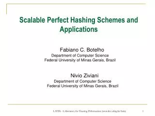
LATIN - LAboratory for Treating INformation (www.dcc.ufmg.br/latin) 1 A Highly Scalable Perfect Hashing Algorithm Nivio Ziviani Fabiano C. Botelho Department of Computer Science Federal University of Minas Gerais, Brazil 3rd Intl. Conference on Scalable Information Systems Naples, Italy, June 4-6, 2008
Objective of the Presentation Present a perfect hashing algorithm: Sequential construction of the function Distributed construction of the function Description and evaluation of the function: Centralized in one machine Distributed among the participating machines Algorithm is highly scalable, time efficient and near space-optimal LATIN - LAboratory for Treating INformation (www.dcc.ufmg.br/latin) 4
LATIN - LAboratory for Treating INformation (www.dcc.ufmg.br/latin) 5 Perfect Hash Function Static key set S of size n ... 0 1 n -1 Hash Table Perfect Hash Function ... m -1 0 1
LATIN - LAboratory for Treating INformation (www.dcc.ufmg.br/latin) 6 Minimal Perfect Hash Function Static key set S of size n ... 0 1 n -1 Minimal Perfect Hash Function Hash Table ... n -1 0 1
The Algorithm A perfect hashing algorithm that uses the idea of partitioning the input key set into small buckets: • Key set fits in the internal memory • Internal Random Access memory algorithm • Key set larger than the internal memory • External Cache-Aware memory algorithm
LATIN - LAboratory for Treating INformation (www.dcc.ufmg.br/latin) 8 Where to use a PHF or a MPHF? • Access items based on the value of a key is ubiquitous in Computer Science • Work with huge static item sets: • In data warehousing applications: • On-Line Analytical Processing (OLAP) applications • In Web search engines: • Large vocabularies • Map long URLs in smaller integer numbers that are used as IDs
LATIN - LAboratory for Treating INformation (www.dcc.ufmg.br/latin) 9 Vocabulary Inverted List Collection of documents Term 1 Doc 1 Doc 5 ... Doc 1 Doc 2 Doc 3 Doc 4 Doc 5 ... Doc n Term 2 Doc 1 Doc 2 ... Term 3 Doc 3 Doc 4 ... Term 4 Doc 7 Doc 9 ... Term 5 Doc 6 Doc 10 ... Term 6 Doc 1 Doc 5 ... Term 7 Term 8 ... Term t Doc 9 Doc 11 ... Indexing: Representing the Vocabulary Indexing
LATIN - LAboratory for Treating INformation (www.dcc.ufmg.br/latin) 10 0 Web Graph Vertices 1 URL 1 URLS 2 URL 2 URL3 3 URL4 URL5 4 URL6 URL7 5 ... 6 URLn ... n-1 Mapping URLs to Web Graph Vertices
LATIN - LAboratory for Treating INformation (www.dcc.ufmg.br/latin) 11 0 Web Graph Vertices M P H F 1 URL 1 URLS 2 URL 2 URL3 3 URL4 URL5 4 URL6 URL7 5 ... 6 URLn ... n-1 Mapping URLs to Web Graph Vertices
Information Theoretical Lower Bounds for Storage Space • PHFs (m ≈ n): • MPHFs (m = n): m < 3n
Related Work • Theoretical Results (use uniform hashing) • Practical Results (use universal hashing - assume uniform hashing for free) • Heuristics
Theoretical ResultsUse Complete Randomness (Uniform Hash Functions) LATIN - LAboratory for Treating INformation (www.dcc.ufmg.br/latin)14
Theoretical ResultsUse Complete Randomness (Uniform Hash Functions) LATIN - LAboratory for Treating INformation (www.dcc.ufmg.br/latin)15
Practical ResultsAssume Uniform Hashing for Free (Use Universal Hashing) LATIN - LAboratory for Treating INformation (www.dcc.ufmg.br/latin)16
Practical ResultsAssume Uniform Hashing for Free (Use Universal Hashing) LATIN - LAboratory for Treating INformation (www.dcc.ufmg.br/latin)17
Practical ResultsAssume Uniform Hashing for Free (Use Universal Hashing) LATIN - LAboratory for Treating INformation (www.dcc.ufmg.br/latin)18
The Sequential External Cache-Aware Algorithm... LATIN - LAboratory for Treating INformation (www.dcc.ufmg.br/latin) 20
LATIN - LAboratory for Treating INformation (www.dcc.ufmg.br/latin) 21 External Cache-Aware Memory Algorithm • First MPHF algorithm for very large key sets (in the order of billions of keys) • This is possible because • Deals with external memory efficiently • Works in linear time • Generates compact functions (near space-optimal) • MPHF (m = n): 3.3n bits • PHF (m =1.23n): 2.7n bits • Theoretical lower bound: • MPHF:1.44n bits • PHF: 0.89n bits
LATIN - LAboratory for Treating INformation (www.dcc.ufmg.br/latin) 22 Sequential External Perfect Hashing Algorithm n-1 0 1 Key Set S … h0 Partitioning Buckets … 0 1 2b - 1 2 Searching MPHF0 MPHF1 MPHF2 MPHF2b-1 Hash Table … n-1 0 1 MPHF(x) = MPHFi(x) + offset[i];
LATIN - LAboratory for Treating INformation (www.dcc.ufmg.br/latin) 23 Key Set Does Not Fit In Internal Memory n-1 0 Key Set S of β bytes ... … ... µ bytes of Internal memory µ bytes of Internal memory Partitioning h0 h0 … … … 0 0 1 2b - 1 1 2b - 1 2 2 File N File 1 Each bucket ≤ 256 N = β/µ b = Number of bits of each bucket address
Important Design Decisions • We map long URLs to a fingerprint of fixed size using a hash function • Use our linear time and near space-optimal algorithm to generate the MPHF of each bucket • How do we obtain a linear time complexity? • Using internal radix sorting to form the buckets • Using a heap of N entries to drive a N-way merge that reads the buckets from disk in one pass
LATIN - LAboratory for Treating INformation (www.dcc.ufmg.br/latin) 25 Algorithm Used for the Buckets: Internal Random Access Memory Algorithm...
Internal Random Access Memory Algorithm • Near space optimal • Evaluation in constant time • Function generation in linear time • Simple to describe and implement • Known algorithms with near-optimal space either: • Require exponential time for construction and evaluation, or • Use near-optimal space only asymptotically, for large n • Acyclic random hypergraphs • Used before by Majewski et all (1996): O(n log n) bits • We proceed differently: O(n) bits (we changed space complexity, close to theoretical lower bound)
Random Hypergraphs (r-graphs) • 3-graph: 1 0 2 3 4 5 • 3-graph is induced by three uniform hash functions
Random Hypergraphs (r-graphs) • 3-graph: h0(jan) = 1 h1(jan) = 3 h2(jan) = 5 1 0 2 3 4 5 • 3-graph is induced by three uniform hash functions
Random Hypergraphs (r-graphs) • 3-graph: h0(jan) = 1 h1(jan) = 3 h2(jan) = 5 1 0 h0(feb) = 1 h1(feb) = 2 h2(feb) = 5 2 3 4 5 • 3-graph is induced by three uniform hash functions
Random Hypergraphs (r-graphs) • 3-graph: h0(jan) = 1 h1(jan) = 3 h2(jan) = 5 1 0 h0(feb) = 1 h1(feb) = 2 h2(feb) = 5 2 3 h0(mar) = 0 h1(mar) = 3 h2(mar) = 4 4 5 • 3-graph is induced by three uniform hash functions • Our best result uses 3-graphs
Acyclic 2-graph Gr: L:Ø h0 1 2 0 3 jan mar apr feb h1 4 5 6 7
Acyclic 2-graph Gr: L: {0,5} h0 1 2 0 3 jan apr feb h1 4 5 6 7
Acyclic 2-graph 0 1 Gr: L: {0,5} {2,6} h0 1 2 0 3 jan apr h1 4 5 6 7
Acyclic 2-graph 0 1 2 Gr: L: {0,5} {2,6} {2,7} h0 1 2 0 3 jan h1 4 5 6 7
Acyclic 2-graph 0 1 2 3 Gr: L: {0,5} {2,6} {2,7} {2,5} h0 1 2 0 3 Gr is acyclic h1 4 5 6 7
Internal Random Access Memory Algorithm (r=2) S jan feb mar apr
Internal Random Access Memory Algorithm (r=2) S Gr: jan feb mar apr h0 1 2 0 3 jan Mapping mar apr feb h1 4 5 6 7
Internal Random Access Memory Algorithm (r=2) g S Gr: 0 r jan feb mar apr r 1 h0 1 2 0 3 r 2 L 3 r jan Mapping Assigning mar apr r feb 4 5 r h1 4 5 6 7 6 r 7 r 0 1 2 3 L: {0,5} {2,6} {2,7} {2,5}
Internal Random Access Memory Algorithm (r=2) g S Gr: 0 r jan feb mar apr r 1 h0 1 2 0 3 0 2 L 3 r jan Mapping Assigning mar apr r feb 4 5 r h1 4 5 6 7 6 r 7 r 0 1 2 3 L: {0,5} {2,6} {2,7} {2,5}
Internal Random Access Memory Algorithm (r=2) g S Gr: 0 r jan feb mar apr r 1 h0 1 2 0 3 0 2 L 3 r jan Mapping Assigning mar apr r feb 4 5 r h1 4 5 6 7 6 r 7 1 0 1 2 3 L: {0,5} {2,6} {2,7} {2,5}
Internal Random Access Memory Algorithm (r=2) g S assigned Gr: assigned 0 0 jan feb mar apr r 1 h0 1 2 0 3 0 2 L 3 r jan Mapping Assigning mar apr r feb 4 5 r h1 4 5 6 7 6 1 7 1 assigned assigned
Internal Random Access Memory Algorithm (r=2) g S assigned Gr: assigned 0 0 jan feb mar apr r 1 h0 1 2 0 3 0 2 L 3 r jan Mapping Assigning mar apr r feb 4 5 r h1 4 5 6 7 6 1 7 1 assigned assigned i = (g[h0(feb)] + g[h1(feb)]) mod r =(g[2] + g[6]) mod 2 = 1
Internal Random Access Memory Algorithm: PHF Hash Table g S assigned Gr: assigned 0 0 mar jan feb mar apr r - 1 h0 1 2 0 3 jan 0 2 L 3 - r jan Mapping Assigning mar apr - r feb 4 5 - r h1 4 5 6 7 6 feb 1 7 apr 1 assigned assigned i = (g[h0(feb)] + g[h1(feb)]) mod r =(g[2] + g[6]) mod 2 = 1 phf(feb) = hi=1 (feb) = 6
Internal Random Access Memory Algorithm: MPHF g S assigned Gr: assigned 0 0 jan feb mar apr Hash Table r 1 h0 1 2 0 3 0 0 mar 2 L 3 jan r 1 jan Mapping Assigning Ranking mar apr 2 feb r feb 4 5 apr r 3 h1 4 5 6 7 6 1 7 1 assigned assigned i = (g[h0(feb)] + g[h1(feb)]) mod r =(g[2] + g[6]) mod 2 = 1 phf(feb) = hi=1 (feb) = 6 mphf(feb) = rank(phf(feb)) = rank(6) = 2
Space to Represent the Function g S Gr: 0 0 jan feb mar apr 2 bits for each entry r 1 h0 1 2 0 3 0 2 L 3 r jan Mapping Assigning mar apr r feb 4 5 r h1 4 5 6 7 6 1 7 1
Space to Represent the Functions (r = 3) • PHF g: [0,m-1] → {0,1,2} • m = cn bits, c = 1.23 → 2.46 n bits • (log 3) cn bits, c = 1.23 → 1.95 n bits (arith. coding) • Optimal: 0.89n bits • MPHF g: [0,m-1] → {0,1,2,3}(ranking info required) • 2m + εm = (2+ ε)cn bits • For c = 1.23 and ε = 0.125 → 2.62 n bits • Optimal: 1.44n bits.
Use of Acyclic Random Hypergraphs • Sufficient condition to work • Repeatedly selects h0, h1..., hr-1 • For r = 3, m = 1.23n: Pra tends to 1 • Number of iterations is 1/Pra = 1
Experimental Results • Metrics: • Generation time • Storage space for the description • Evaluation time • Collection: • 1.024 billions of URLs collected from the web • 64 bytes long on average • Experiments • Commodity PC with a cache of 4 Mbytes • 1.86 GHz, 1 GB, Linux, 64 bits architecture
Related Algorithms • Fox, Chen and Heath (1992) – FCH • Majewski, Wormald, Havas and Czech (1996) – MWHC All algorithms coded in the same framework