Download
1 / 46
470 likes | 709 Vues
Bahan kajian MK Perencanaan Lingkungan, soemarno desember 2011. MULTI-CRITERIA ANALYSIS PENGELOLAAN DAERAH ALIRAN SUNGAI. MULTIPLE GOALS PROGRAMMING. http://www.kswraps.org/planning. Goal Programming

E N D
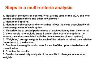
Bahan kajian MK Perencanaan Lingkungan, soemarno desember 2011 MULTI-CRITERIA ANALYSIS PENGELOLAAN DAERAH ALIRAN SUNGAI MULTIPLE GOALS PROGRAMMING
Goal Programming Goal programming is a branch of multiple objective programming, which in turn is a branch of multi-criteria decision analysis (MCDA), also known as multiple-criteria decision making (MCDM). It can be thought of as an extension or generalisation of linear programming to handle multiple, normally conflicting objective measures (ukuran/dimensi dari tujuan).
Each of these measures is given a goal or target value to be achieved. Unwanted deviations from this set of target values are then minimised in an achievement function. This can be a vector or a weighted sum dependent on the goal programming variant used. As satisfaction of the target is deemed to satisfy the decision maker(s), an underlying satisficing philosophy is assumed.
Variants The initial goal programming formulations ordered the unwanted deviations into a number of priority levels, with the minimisation of a deviation in a higher priority level being of infinitely more importance than any deviations in lower priority levels. (penetapan prioritas goals) This is known as Lexicographic or pre-emptive Goal Programming.
Lexicographic goal programming Ignizio gives an algorithm showing how a lexicographic goal programme can be solved as a series of linear programmes. Lexicographic goal programming should be used when there exists a clear priority ordering amongst the goals to be achieved.
If the decision maker is more interested in direct comparisons of the objectives ……… ……then Weighted Goal Programming should be used. (penetapan bobot untuk masing-masing goal) In this case all the unwanted deviations are multiplied by weights, reflecting their relative importance, and added together as a single sum to form the achievement function.
It is important to recognise that deviations measured in different units cannot be summed directly due to the phenomenon of incommensurability. Hence each unwanted deviation is multiplied by a normalisation constant to allow direct comparison. (normalisasi dilakukan untuk dapat membandingkan simpangan ketidak-tercapaian goals)
Popular choices for normalisation constants are the goal target value of the corresponding objective (hence turning all deviations into percentages) or the range of the corresponding objective (between the best and the worst possible values, hence mapping all deviations onto a zero-one range) .
For decision makers more interested in obtaining a balance between the competing objectives, Chebyshev Goal Programming should be used. Introduced by Flavell in 1976 [9], this variant seeks to minimise the maximum unwanted deviation, rather than the sum of deviations. (MEMINIMUMKAN SIMPANGAN DARI KENDALA TUJUAN TERTENTU YANG TIDAK DIINGINKAN) This utilises the Chebyshev distance metric, which emphasizes justice and balance rather than ruthless optimisation.
Kekuatan dan Kelemahan A major strength of goal programming is its simplicity and ease of use. This accounts for the large number of goal programming applications in many and diverse fields . As weighted and Chebyshev goal programmes can be solved by widely available linear programming computer packages, finding a solution tool is not difficult in most cases. Lexicographic goal programmes can be solved as a series of linear programming models, as described by Ignizio and Cavalier .
Goal programming Goal programming can hence handle relatively large numbers of variables, constraints and objectives. A debated weakness is the ability of goal programming to produce solutions that are not Pareto efficient. This violates a fundamental concept of decision theory, that is no rational decision maker will knowingly choose a solution that is not Pareto efficient.
Analytic Hierarchy Process However, techniques are available to detect when this occurs and project the solution onto the Pareto efficient solution in an appropriate manner. The setting of appropriate weights in the goal programming model is another area that has caused debate, with some authors suggesting the use of the Analytic Hierarchy Process or interactive methods for this purpose.
Pengembangan wilayah aliran sungai SISTEM PERTANIAN BERWAWASAN LINGKUNGAN Pembangunan pertanian, menimbulkan dampak lingkungan (DAL): 1. Kebutuhan manusia atas barang dan jasa: Beragam sumberdaya input Gangguan lingkungan 2. Pertumbuhan penduduk: Kegiatan ekonomi pd kondisi lingkungan rawan 3. Pengembangan teknologi ---------------- DAL 4. Mekanisme pasar ------------- Mengabaikan biaya sosial 5. Peningkatan produksi --- LIMBAH --- Kualitas Lingkn 6. DAS ------------- Ekosistem Pertanian yang Tipikal
http://www.sfei.org/wetlands/Rep...ject.pdf of the Arkansas Watershed
KONFIGURASI DAS Ecological yield: Debit air, sedimen Economic yield: Bio-economic yield, ton/ha Cash income, rp/ha Employment, HOK/th/ha Sub DAS I III II IV V VI VII X VIII x6 X2 x4 X1 x5 IX X3
http://www.kars.ku.edu/research/...ability/ Watershed Classification System
Pengembangan wilayah aliran sungai MGP: Multiple Goal Programming Teknik pemrograman matematika untuk menyelesaikan maslaah pengambilan keputusan yang mempunyai beberapa tujuan yang tidak dapat dipenuhi secara serempak Tahapan: Problem identification Tahapan: Problem solving Identifikasi Masalah: 1. Diagram lingkar sebab-akibat (causal loop diagram) 1.1. Semua peubah yang berperan 1.2. Pengaruh peubah thd yang lain …………… tanda panah 1.3. Sifat pengaruh/ akibat ……………. tanda + atau – 2. Diagram Kotak Hitam: Input SISTEM Output Proses-proses
Pengembangan wilayah aliran sungai DAS -------------------- Aktivitas manusia: 1. Konstruksi fisik (X1) 2. Pertambangan (X2) 3. Pertanian (X3) 4. Perikanan (X4) 5. Peternakan (X5) 6. Perkebunan (X6) 7. Kehutanan (X7) 8. Lainnya (Xi) Dampak Negatif Model Perencanaan 1. Model Optimasi --------untuk mencapai tujuan yg ditetapkan: 2. Model Non-Optimasi 1. Tunggal (single) 2. Ganda (Multiple)
CAUSAL LOOP: Model Perencanaan DAS Evapo- Transpirasi Intersepsi Transpirasi + + Bahan Organik Fisika Tanah Biomasa Vegetasi Dispersi agregat Retensi Air Infiltrasi Penutupan Vegetasi KAT + EROSI Run-off Perkolasi + Konservasi Fluktuasi debit sungai DEBIT Lahan pertanian Intensifikasi Usahatani Produktivitas lahan
Diagram Kotak Hitam Model DAS Geomorfologi Sistem DAS Hidrologi Erosi Hidrologi Sedimentasi Produksi Prod. Lahan Input tak terkontrol Iklim Output Landuse optimum Input terkontrol landuse Parameter DAS Pengelolaan: Konservasi & Intensifikasi
Pengembangan wilayah aliran sungai • Pemecahan masalah: • 1. Analisis Optimasi Landuse: Model MGP • Landuse optimal: Kombinasi optimum dari berbagai jenis landuse • Variabel : Luasan sutu jenis landuse • Ciri utama MGP: • Sasaran yg ingin dicapai diberi urutan prioritas, • setidaknya dalam sekala ORDINAL • 2. Pemenuhan sasaran dilakukan berdasarkan prioritas. Sasaran dengan prioritas lebih rendah baru diperhatikan bila sasaran dg prioritas lebih tinggi telah terpenuhi • 3. Sasaran tidak perlu harus terpenuhi, tetapi diusahakan sedekat mungkin.
Model Umum MGP: a. Fungsi Tujuan Minimumkan Fungsi Tujuan: Z = Σ PkΣ ( w-ki.di- + w+ki .di+ ) b. Fungsi Kendala: Kendala Riil: Σ Σ akj Xj≤ atau ≥ Ck Kendala Sasaran: Σ Σ eij Xj + di- - di+ = bi Xj, di-, di+≥ 0 Dimana: i = 1 …………..m j = 1 ………….. n k = 1………….. p
Pengembangan wilayah aliran sungai Keterangan: Xj : Peubah keputusan ke-j atau kegiatan sub-tujuan eij : Koefisien Xj pada kendala sasaran ke-i akj : Koefisien Xj pada kendala sasaran ke-k Ck : Nilai kendala riil ke-k, Jumlah sumberdaya ke-k yang tersedia bi : Target sasaran ke-i (RHS) di- : Kekurangan dari sasaran ke i (simpangan negatif) Pk : Faktor prioritas ordinal ke k di+ : Kelebihan dari sasaran ke i Wki- : bobot bagi di- pada prioritas Pk Wki+ : Bobot bagi di+ pada prioritas Pk
Peubah dan Parameter: Peubah (Xi): X1 : Luas hutan (ha) X2 : Luas tanaman tahunan lahan kering (ha) X3 : Luas tanaman pangan lahan kering (ha) X4 : Luas padi sawah (ha) X5 : Luas alang-alang (ha) X6 : Luas pemukiman (ha). Parameter (Sasaran = RHS) a1 s/d a10: Debit /limpasan permukaan bulanan sub DAS ke 1 s/d 10 (m3) a11 s/d a20: Kehilangan tanah tolerable pd sub DAS ke 1 s/d 10 (mm/th) a21 s/d a30 : Sediment Delivery Ratio (SDR) pada sub DAS ke 1 s/d 10 a31 s/d a40 : Trapping efficiency (TE) pada sub DAS ke-1 s/d 10
Pengembangan wilayah aliran sungai Parameter: a41 : Produktivitas hutan a42 : Produktivitas kebun tanaman tahunan , kw/ha a43 : Produktivitas tegal tranaman pangan, kw/ha a44 : Produktivitas padi sawah , kw/ha a45 – a54 : Pendapatan petani sub DAS ke 1 s/d ke 10, rp/ha/th a55 : Rasio min. luas hutan dg luas DAS yg diinginkan a56 : Rasio minimum luas kebun dengan luas DAS a57 : Rasio minimum luas tegalan dengan luas DAS a58 : Rasio minimum luas sawah dengan luas DAS a59 : Rasio minimum luas alang-alang dngan luas DAS a60 : Rasio minimum luas pemukiman dngan luas DAS
Pengembangan wilayah aliran sungai • Fungsi Kendala Model: Urutan Prioritas • 1. Kendala luas landuse • 2. p1: Kendala sasaran debit atau runoff • 3. p2: Kendala sasaran toleransi erosi • 4. p3: Kendala sasaran sedimentasi minimum • p3: Kendala sasaran produksi usahatani • p4 : Kendala sasaran total income petani • (p1 : prioritas tinggi, p4: prioritas rendah) • Fungsi Tujuan Model: • Z = p1 Σdk- + p2 Σ dk+ + p3 Σ dk+ + p4 Σ dk-
Fungsi Kendala: Kendala riil luas lahan: DAS = 10 Sub DAS 1. Luas Hutan (X1) e1X1.1 + e2 X1.2 + …………..+ e10X1.10 + d1- = X1 2. Luas Kebun (X2) e1X2.1 + e2 X2.2 + …………..+ e10X2.10 + d2- = X2 3. Luas Tegalan (X3) e1X3.1 + e2 X3.2 + ………..+ e10X3.10 + d3- = X3 ………. Dst…… 6. Luas Permukiman (X6) e1X6.1 + e2 X6.2 + ………..+ e10 X6.10 + d6- = X6 7. Kendala sasaran Debit:
Kendala sasaran Debit atau run off: 7. Sub DAS 1 e17 X17 + ………………… + e67 X67 + d7- = a1 8. Sub DAS 2 : e18 X18 + ………………… + e68 X68 + d8- = a2 ………dst…….. 16. Sub DAS 10: e1.16 X1.16 + ………………… + e6.16 X6.16 + d16- = a10 X1.7 = luas lahan pada sub DAS 1 X1.16 = luas lahan pada sub DAS 10 X6.7 = luas permukiman pada sub DAS 1 Dst….
Fungsi kendala riil / sasaran 1. X1.1 + X2.1 + X3.1 + X4.1 + X5.1 + X6.1 = Ck1
ANALISIS HIDROLOGIS A. HIDROLOGI Model: Q = a. Qmaks (1-ekt ) Peubah yg ditetapkan / dipilih : 1. Laju transpirasi Dimana: 2. Besaran intersepsi Q= Peubah yang ditetapkan (1-4) 3. Laju evaporasi dari tanah Qmaks= NIlai maksimum dari Q 4. Laju evaporasi permukaan air bebas a= Faktor koreksi bagi Q t= Peubah bebas k= Konstante e= Bilangan alam
b. EROSI Model: A = R.K.L.S.C.P. A : Kehilangan tanah, ton/ha/th R : Faktor erosivitas hujan K : Faktor reodibilitas tanah Dst……… Toleransi erosi tanah: Tolerable Soil Loss TSL = (SDE x SDF) / T SDE : Kedalaman efektif tanah, mm SDF : Faktor kedalaman tanah.
c. TINGKAT SEDIMENTASI Sedimen Potensial = (Erosi aktual) x SDR Sedimen Erosi Aktual yang masuk ke sungai SDR = -------------------------------------------------------- Volume sedimen di lahan d. PRODUKTIVITAS LAHAN 1. Usahatani Sawah 2. Usahatani Tegalan 3. Usahatani Kebun 4. Produksi Hutan e. INCOME PETANI: ∏ = TP - TC ∏ : Income usahatani TP : Total produksi TC : Total biaya produksi