Download
1 / 51
510 likes | 521 Vues
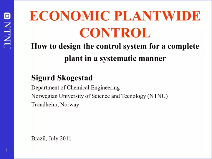
ECONOMIC PLANTWIDE CONTROL How to design the control system for a complete plant in a systematic manner. Sigurd Skogestad Department of Chemical Engineering Norwegian University of Science and Tecnology (NTNU) Trondheim, Norway Brazil, July 2011. Plantwide control lectures. Sigurd Skogestad.

E N D
ECONOMIC PLANTWIDE CONTROLHow to design the control system for a complete plant in a systematic manner Sigurd Skogestad Department of Chemical Engineering Norwegian University of Science and Tecnology (NTNU) Trondheim, Norway Brazil, July 2011
Plantwide control lectures. Sigurd Skogestad Outline (6 lectures) • Control structure design (plantwide control) • A procedure for control structure design I Top Down • Step S1: Define operational objective (cost) and constraints • Step S2: Identify degrees of freedom and optimize operation for disturbances • Step S3: Implementation of optimal operation • What to control ? (primary CV’s) (self-optimizing control) • Step S4: Where set the production rate? (Inventory control) II Bottom Up • Step S5: Regulatory control: What more to control (secondary CV’s) ? • Distillation column control • Step S6: Supervisory control • Step S7: Real-time optimization • PID tuning • (+ decentralized control if time) Lecture 1* (49) Lecture 2 (71)+ Lecture 3 (36) Lecture 4 (62)+ Lecture 5 (19) Lecture 6 (54) *Each lecture is 2 hours with a 10 min intermediate break after about 55 min (no. of slides) + means that it most likely will continue into the next lecture
Main references • The following paper summarizes the procedure: • S. Skogestad, ``Control structure design for complete chemical plants'', Computers and Chemical Engineering, 28 (1-2), 219-234 (2004). • There are many approaches to plantwide control as discussed in the following review paper: • T. Larsson and S. Skogestad, ``Plantwide control: A review and a new design procedure'' Modeling, Identification and Control, 21, 209-240 (2000). • The following paper updates the procedure: • S. Skogestad, ``Economic plantwide control’’, Book chapter in V. Kariwala and V.P. Rangaiah (Eds), Plant-Wide Control: Recent Developments and Applications”, Wiley (late 2011). http://www.nt.ntnu.no/users/skoge/publications/2011/skogestad-plantwide-control-book-by-kariwala/ All papers available at: http://www.nt.ntnu.no/users/skoge/
S. Skogestad ``Plantwide control: the search for the self-optimizing control structure'',J. Proc. Control, 10, 487-507 (2000). • S. Skogestad, ``Self-optimizing control: the missing link between steady-state optimization and control'',Comp.Chem.Engng., 24, 569-575 (2000). • I.J. Halvorsen, M. Serra and S. Skogestad, ``Evaluation of self-optimising control structures for an integrated Petlyuk distillation column'',Hung. J. of Ind.Chem., 28, 11-15 (2000). • T. Larsson, K. Hestetun, E. Hovland, and S. Skogestad, ``Self-Optimizing Control of a Large-Scale Plant: The Tennessee Eastman Process'',Ind. Eng. Chem. Res., 40 (22), 4889-4901 (2001). • K.L. Wu, C.C. Yu, W.L. Luyben and S. Skogestad, ``Reactor/separator processes with recycles-2. Design for composition control'', Comp. Chem. Engng., 27 (3), 401-421 (2003). • T. Larsson, M.S. Govatsmark, S. Skogestad, and C.C. Yu, ``Control structure selection for reactor, separator and recycle processes'', Ind. Eng. Chem. Res., 42 (6), 1225-1234 (2003). • A. Faanes and S. Skogestad, ``Buffer Tank Design for Acceptable Control Performance'', Ind. Eng. Chem. Res., 42 (10), 2198-2208 (2003). • I.J. Halvorsen, S. Skogestad, J.C. Morud and V. Alstad, ``Optimal selection of controlled variables'', Ind. Eng. Chem. Res., 42 (14), 3273-3284 (2003). • A. Faanes and S. Skogestad, ``pH-neutralization: integrated process and control design'', Computers and Chemical Engineering, 28 (8), 1475-1487 (2004). • S. Skogestad, ``Near-optimal operation by self-optimizing control: From process control to marathon running and business systems'', Computers and Chemical Engineering, 29 (1), 127-137 (2004). • E.S. Hori, S. Skogestad and V. Alstad, ``Perfect steady-state indirect control'', Ind.Eng.Chem.Res, 44 (4), 863-867 (2005). • M.S. Govatsmark and S. Skogestad, ``Selection of controlled variables and robust setpoints'', Ind.Eng.Chem.Res, 44 (7), 2207-2217 (2005). • V. Alstad and S. Skogestad, ``Null Space Method for Selecting Optimal Measurement Combinations as Controlled Variables'', Ind.Eng.Chem.Res, 46 (3), 846-853 (2007). • S. Skogestad, ``The dos and don'ts of distillation columns control'', Chemical Engineering Research and Design (Trans IChemE, Part A), 85 (A1), 13-23 (2007). • E.S. Hori and S. Skogestad, ``Selection of control structure and temperature location for two-product distillation columns'', Chemical Engineering Research and Design (Trans IChemE, Part A), 85 (A3), 293-306 (2007). • A.C.B. Araujo, M. Govatsmark and S. Skogestad, ``Application of plantwide control to the HDA process. I Steady-state and self-optimizing control'', Control Engineering Practice, 15, 1222-1237 (2007). • A.C.B. Araujo, E.S. Hori and S. Skogestad, ``Application of plantwide control to the HDA process. Part II Regulatory control'', Ind.Eng.Chem.Res, 46 (15), 5159-5174 (2007). • V. Lersbamrungsuk, T. Srinophakun, S. Narasimhan and S. Skogestad, ``Control structure design for optimal operation of heat exchanger networks'', AIChE J., 54 (1), 150-162 (2008). DOI 10.1002/aic.11366 • 990-999 (2008). T. Lid and S. Skogestad, ``Data reconciliation and optimal operation of a catalytic naphtha reformer'', Journal of Process Control, 18, 320-331 (2008). • E.M.B. Aske, S. Strand and S. Skogestad, ``Coordinator MPC for maximizing plant throughput'', Computers and Chemical Engineering, 32, 195-204 (2008). • A. Araujo and S. Skogestad, ``Control structure design for the ammonia synthesis process'', Computers and Chemical Engineering, 32 (12), 2920-2932 (2008). • E.S. Hori and S. Skogestad, ``Selection of controlled variables: Maximum gain rule and combination of measurements'', Ind.Eng.Chem.Res, 47 (23), 9465-9471 (2008). • V. Alstad, S. Skogestad and E.S. Hori, ``Optimal measurement combinations as controlled variables'', Journal of Process Control, 19, 138-148 (2009) • E.M.B. Aske and S. Skogestad, ``Consistent inventory control'', Ind.Eng.Chem.Res, 48 (44), 10892-10902 (2009). + MORE
Practice: Tennessee Eastman challenge problem (Downs, 1991)(“PID control”)
How we design a control system for a complete chemical plant? • How do we get from PID control to PhD control? • Where do we start? • What should we control? and why? • etc. • etc.
Alan Foss (“Critique of chemical process control theory”, AIChE Journal,1973): The central issue to be resolved ... is the determination of control system structure. Which variables should be measured, which inputs should be manipulated and which links should be made between the two sets? There is more than a suspicion that the work of a genius is needed here, for without it the control configuration problem will likely remain in a primitive, hazily stated and wholly unmanageable form. The gap is present indeed, but contrary to the views of many, it is the theoretician who must close it. • Carl Nett (1989): Minimize control system complexity subject to the achievement of accuracy specifications in the face of uncertainty.
Control structure design • Not the tuning and behavior of each control loop, • But rather the control philosophy of the overall plant with emphasis on the structural decisions: • Selection of controlled variables (“outputs”) • Selection of manipulated variables (“inputs”) • Selection of (extra) measurements • Selection of control configuration (structure of overall controller that interconnects the controlled, manipulated and measured variables) • Selection of controller type (LQG, H-infinity, PID, decoupler, MPC etc.). • That is:Control structure design includes all the decisions we need make to get from ``PID control’’ to “PhD” control
Process control:“Plantwide control” = “Control structure design for complete chemical plant” • Large systems • Each plant usually different – modeling expensive • Slow processes – no problem with computation time • Structural issues important • What to control? Extra measurements, Pairing of loops • Previous work on plantwide control: • Page Buckley (1964) - Chapter on “Overall process control” (still industrial practice) • Greg Shinskey (1967) – process control systems • Alan Foss (1973) - control system structure • Bill Luyben et al. (1975- ) – case studies ; “snowball effect” • George Stephanopoulos and Manfred Morari (1980) – synthesis of control structures for chemical processes • Ruel Shinnar (1981- ) - “dominant variables” • Jim Downs (1991) - Tennessee Eastman challenge problem • Larsson and Skogestad (2000): Review of plantwide control
Control structure selection issues are identified as important also in other industries. Professor Gary Balas (Minnesota) at ECC’03 about flight control at Boeing: The most important control issue has always been to select the right controlled variables --- no systematic tools used!
Main objectives control system • Stabilization • Implementation of acceptable (near-optimal) operation ARE THESE OBJECTIVES CONFLICTING? • Usually NOT • Different time scales • Stabilization fast time scale • Stabilization doesn’t “use up” any degrees of freedom • Reference value (setpoint) available for layer above • But it “uses up” part of the time window (frequency range)
Main simplification: Hierarchical structure Process control RTO Need to define objectives and identify main issues for each layer MPC PID
Dealing with complexity Main simplification: Hierarchical decomposition The controlled variables (CVs) interconnect the layers OBJECTIVE Min J (economics); MV=y1s RTO cs = y1s Follow path (+ look after other variables) CV=y1 (+ u); MV=y2s MPC y2s Stabilize + avoid drift CV=y2; MV=u PID u (valves)
Hierarchical decomposition Example: Bicycle riding Note: design starts from the bottom • Regulatory control: • First need to learn to stabilize the bicycle • CV = y2 = tilt of bike • MV = body position • Supervisory control: • Then need to follow the road. • CV = y1 = distance from right hand side • MV=y2s • Usually a constant setpoint policy is OK, e.g. y1s=0.5 m • Optimization: • Which road should you follow? • Temporary (discrete) changes in y1s
Plantwide control decisions • No matter what procedure we choose to use, the following decisions must be made when designing a plantwide control strategy: • Decision 1. Select ”economic” (primary) controlled variables (CV1) for the supervisory control layer (the setpoints CV1s link the optimization layer with the control layers). • Decision 2. Select ”stabilizing” (secondary) controlled variables (CV2) for the regulatory control layer (the setpoints CV2s link the two control layers). • Decision 3. Locate the throughput manipulator (TPM). • Decision 4. Select pairings for the stabilizing layer, that is, pair inputs (valves) and controlled variables (CV2). By “valves” is here meant the original dynamic manipulated variables.
y1 y2 MVs Process Skogestad plantwide control structure design procedure I Top Down • Step S1: Define operational objectives (optimal operation) • Cost function J (to be minimized) • Operational constraints • Step S2 (optimization): (a) Identify degrees of freedom (MVs). (b) Optimize for expected disturbances and find regions of active constraints • Step S3 (implementation): Select primary controlled variables c=y1 (CVs) (Decision 1). • Step S4: Where set the production rate? (Inventory control) (Decision 3) II Bottom Up • Step S5: Regulatory / stabilizing control (PID layer) • What more to control (y2; local CVs)? y (Decision 2) • Pairing of inputs and outputs y (Decision 4) • Step S6: Supervisory control (MPC layer) • Step S7: Real-time optimization (Do we need it?) Understanding and using this procedure is the most important part of this course!!!!
Comment: Luyben procedure • Step L1. Establish control objectives • Step L2. Determine control degrees of freedom • Step L3. Establish energy management system • Step L4. Set the production rate (Decision 3) • Step L5. Control product quality and handle safety, environmental and operational constraints • Step L6. Fix a flow in every recycle loop and control inventories • Step L7. Check component balances • Step L8. Control individual unit operations • Step L9.Optimize economics and improve dynamic controllability Notes: • “Establish control objectives” in step L1 does not lead directly to the choice of controlled variables (Decisions 1 and 2). Thus, in Luyben’s procedure, Decisions 1, 2 and 4 are not explicit, but are included implicitly in most of the steps. • Even though the procedure is systematic, it is still heuristic and ad hoc in the sense that it is not clear how the authors arrived at the steps or their order. • A major weakness is that the procedure does not include economics, except as an afterthought in step L9.
Outline • Skogestad procedure for control structure design I Top Down • Step S1: Define operational objective (cost) and constraints • Step S2: Identify degrees of freedom and optimize operation for disturbances • Step S3: Implementation of optimal operation • What to control ? (primary CV’s) (self-optimizing control) • Step S4: Where set the production rate? (Inventory control) II Bottom Up • Step S5: Regulatory control: What more to control (secondary CV’s) ? • Step S6: Supervisory control • Step S7: Real-time optimization
Step S1. Define optimal operation (economics) • What are we going to use our degrees of freedom u(MVs) for? • Define scalar cost function J(u,x,d) • u: degrees of freedom (usually steady-state) • d: disturbances • x: states (internal variables) Typical cost function*: • Optimize operation with respect to u for given d (usually steady-state): minu J(u,x,d) subject to: Model equations: f(u,x,d) = 0 Operational constraints: g(u,x,d) < 0 J = cost feed + cost energy – value products *No need to include fixed costs (capital costs, operators, maintainance) at ”our” time scale (hours) Note: Operational profit P = -J.
Optimal operation distillation column • Distillation at steady state with given p and F: N=2 DOFs, e.g. L and V (u) • Cost to be minimized (economics) J = - P where P= pD D + pB B – pF F – pV • Constraints Purity D: For example xD, impurity· max Purity B: For example, xB, impurity· max Flow constraints: min · D, B, L etc. · max Column capacity (flooding): V · Vmax, etc. Pressure: 1) p given (d) 2) p free (u): pmin· p · pmax Feed: 1) F given (d) 2) F free (u): F · Fmax • Optimal operation: Minimize J with respect to steady-state DOFs (u) cost energy (heating+ cooling) value products cost feed
Outline • Skogestad procedure for control structure design I Top Down • Step S1: Define operational objective (cost) and constraints • Step S2: Identify degrees of freedom and optimize operation for disturbances • Step S3: Implementation of optimal operation • What to control ? (primary CV’s) (self-optimizing control) • Step S4: Where set the production rate? (Inventory control) II Bottom Up • Step S5: Regulatory control: What more to control (secondary CV’s) ? • Step S6: Supervisory control • Step S7: Real-time optimization
Step S2 (Optimize operation):(a) Identify degrees of freedom (b) Optimize for expected disturbances • Need good steady-state model • Goal: Identify regions of active constraints • Time consuming!
Plans for next lectures • Step 2 (Find optimal operation using offline calculations): • Step 2a : DOF analysis (steady-state) (12 slides) • Step 2b: Optimize for expected disturbances (1 slide) • QUIZ’s • Step 3 (Implementation of optimal operation) (Lecture 2, many slides!) Identify primary (“economic”) controlled variables (CVs): • Control active constraints. Backoff • Remaining unconstrained: Find “self-optimizing” CVs Will use a lot of time on this!
Steady-state DOFs Step S2a: Degrees of freedom (DOFs) for operation NOT as simple as one may think! To find all operational (dynamic) degrees of freedom: • Count valves! (Nvalves) • “Valves” also includes adjustable compressor power, etc. Anything we can manipulate! BUT: not all these have a (steady-state) effect on the economics
Steady-state DOFs Steady-state degrees of freedom (DOFs) IMPORTANT! DETERMINES THE NUMBER OF VARIABLES TO CONTROL! • No. of primary CVs = No. of steady-state DOFs Methods to obtain no. of steady-state degrees of freedom (Nss): • Equation-counting • Nss = no. of variables – no. of equations/specifications • Very difficult in practice • Valve-counting (easier!) • Nss = Nvalves – N0ss – Nspecs • N0ss = variables with no steady-state effect • Potential number for some units (useful for checking!) • Correct answer: Will eventually find it when we perform optimization CV = controlled variable (c)
Steady-state DOFs Steady-state degrees of freedom (Nss): 2. Valve-counting • Nvalves = no. of dynamic (control) DOFs (valves) • Nss = Nvalves – N0ss – Nspecs : no. of steady-state DOFs • N0ss = N0y + N0,valves : no. of variables with no steady-state effect • N0,valves : no. purely dynamic control DOFs • N0y : no. controlled variables (liquid levels) with no steady-state effect • Nspecs: No of equality specifications (e.g., given pressure)
Steady-state DOFs Typical Distillation column 4 5 3 1 With given feed and pressure: NEED TO IDENTIFY 2 more CV’s - Typical: Top and btm composition 6 2 Nvalves = 6 , N0y = 2* , NDOF,SS = 6 -2 = 4 (including feed and pressure as DOFs) *N0y: no. controlled variables (liquid levels) with no steady-state effect
Steady-state DOFs QUIZ 3 Heat-integrated distillation process
Steady-state DOFs Heat exchanger with bypasses
Steady-state DOFs Steady-state degrees of freedom (Nss): 3. Potential number for some process units • each external feedstream: 1 (feedrate) • splitter: n-1 (split fractions) where n is the number of exit streams • mixer: 0 • compressor, turbine, pump: 1 (work/speed) • adiabatic flash tank: 0* • liquid phase reactor: 1 (holdup reactant) • gas phase reactor: 0* • heat exchanger: 1 (bypass or flow) • column (e.g. distillation) excluding heat exchangers: 0*+ no. of sidestreams • pressure* : add 1DOF at each extra place you set pressure (using an extra valve, compressor or pump), e.g. in adiabatic flash tank, gas phase reactor or absorption column • *Pressure is normally assumed to be given by the surrounding process and is then not a degree of freedom • Ref: Araujo, Govatsmark and Skogestad (2007) • Extension to closed cycles: Jensen and Skogestad (2009) • Real number may be less, for example, if there is no bypass valve
Steady-state DOFs Heat exchanger with bypasses
Steady-state DOFs Distillation column (with feed and pressure as DOFs) split “Potential number”, Nss= 0 (column distillation) + 1 (feed) + 2*1 (heat exchangers) + 1 (split) = 4 With given feed and pressure: N’ss = 4 – 2 = 2
Steady-state DOFs Heat-integrated distillation process
Steady-state DOFs Purge (H2 + CH4) Compressor H2 + CH4 Toluene Quench Mixer FEHE Furnace PFR Separator Cooler CH4 Toluene Benzene Toluene Column Stabilizer Benzene Column Diphenyl QUIZ 4 HDA process
Steady-state DOFs QUIZ 4 solution HDA process: steady-state degrees of freedom 8 7 • Hm….. Consider • Feeds • Heat exchangers • Splitters • Compressors • Distillation columns feed:1.2 hex: 3, 4, 6 splitter 5, 7 compressor: 8 distillation: 2 each column 3 1 2 4 5 6 13 11 9 Conclusion: 14 steady-state DOFs 14 12 10 Assume given column pressures
Steady-state DOFs • Check that there are enough manipulated variables (DOFs) - both dynamically and at steady-state (step 2) • Otherwise: Need to add equipment • extra heat exchanger • bypass • surge tank
Step S2b: Optimize with respects to DOFS (u) for expected disturbances (d) …….. and identify regions of active constraints minu J(u,x,d) subject to: Model equations: f(u,x,d) = 0 Operational constraints: g(u,x,d) < 0 • Idea: Prepare operation for expected future disturbances, incl. price changes • In principle: simple • In practise: very time consuming • Commercial simulators (Aspen, Unisim/Hysys) are set up in “design mode” and often work poorly in “operation (rating) mode”. • Example Heat exchanger • Easy (Design mode): Given streams (and temperatures), find UA • Difficult (Operation mode): Given UA, find outlet temperatures • Optimization methods in commercial simulators often poor • We use Matlab or even Excel “on top” • Heat exchanger: Let Matlab/Excel vary temperatures to match given UA • Focus on most important disturbances and range. Whole picture is complicated d2 = energy price d1 = feedrate Ref. Jacobsen and Skogestad, ESCAPE’21, Greece, 2011
Optimal operation minimize J = cost feed + cost energy – value products Mode 1. Given feedrate Mode 2. Maximum production Two main cases (modes) depending on marked conditions:
Mode 1. Given feedrate Amount of products is then usually indirectly given and Optimal operation is then usually unconstrained J = cost feed– value products + cost energy constant “maximize efficiency (energy)” Control: Operate at optimal trade-off (not obvious what to control to achieve this) J = energy c copt
J Infeasible region c copt Mode 2. Maximum production J = cost feed + cost energy – value products • Assume feedrate is degree of freedom • Assume products much more valuable than feed • Optimal operation is then to maximize product rate • But must remain feasible • constrained by bottleneck Control: Focus on tight control of bottleneck (“obvious what to control”)
Example with Quiz:Optimal operation of two distillation columns in series
QUIZ 1 Operation of Distillation columns in seriesWith given F (disturbance): 4 steady-state DOFs (e.g., L and V in each column) N=41 αAB=1.33 N=41 αBC=1.5 > 95% B pD2=2 $/mol > 95% A pD1=1 $/mol F ~ 1.2mol/s pF=1 $/mol < 4 mol/s < 2.4 mol/s > 95% C pB2=1 $/mol Cost (J) = - Profit = pF F + pV(V1+V2) – pD1D1 – pD2D2 – pB2B2 Energy price: pV=0-0.2 $/mol (varies) QUIZ: What are the expected active constraints? 1. Always. 2. For low energy prices. DOF = Degree Of Freedom Ref.: M.G. Jacobsen and S. Skogestad (2011)
SOLUTION QUIZ 1 1. xB = 95% B Spec. valuable product (B): Always active! Why? “Avoid product give-away” 2. Cheap energy: V1=4 mol/s, V2=2.4 mol/s Max. column capacity constraints active! Why? Overpurify A & C to recover more B Operation of Distillation columns in seriesWith given F (disturbance): 4 steady-state DOFs (e.g., L and V in each column) Hm….? N=41 αAB=1.33 N=41 αBC=1.5 > 95% B pD2=2 $/mol > 95% A pD1=1 $/mol F ~ 1.2mol/s pF=1 $/mol < 4 mol/s < 2.4 mol/s > 95% C pB2=1 $/mol Cost (J) = - Profit = pF F + pV(V1+V2) – pD1D1 – pD2D2 – pB2B2 Energy price: pV=0-0.2 $/mol (varies) QUIZ: What are the expected active constraints? 1. Always. 2. For low energy prices. DOF = Degree Of Freedom Ref.: M.G. Jacobsen and S. Skogestad (2011)
SOLUTION QUIZ 1 (more details) Active constraint regions for two distillation columns in series Energy price [$/mol] BOTTLENECK Higher F infeasible because all 5 constraints reached [mol/s] CV = Controlled Variable
QUIZ 2 Active constraint regions for two distillation columns in series Energy price [$/mol] [mol/s] QUIZ. Assume low energy prices (pV=0.01 $/mol). How should we control the columns? CV = Controlled Variable
QUIZ 2 Control of Distillation columns in series PC PC LC LC Given LC LC QUIZ. Assume low energy prices (pV=0.01 $/mol). How should we control the columns? HINT: CONTROL ACTIVE CONSTRAINTS Red: Basic regulatory loops
SOLUTION QUIZ 2 Control of Distillation columns in series PC PC LC LC Hm……. HINT: CONTROL ACTIVE CONSTRAINTS! xB CC xBS=95% • 1 unconstrained DOF (L1): • Use for what?? CV=? • Not: CV= xA in D1! (why? xA should vary with F!) • Maybe: constant L1? (CV=L1) • Better: CV= xA in B1? Self-optimizing? Given MAX V2 MAX V1 General for remaining unconstrained DOFs: LOOK FOR “SELF-OPTIMIZING” CVs = Variables we can keep constant WILL GET BACK TO THIS! LC LC QUIZ. Assume low energy prices (pV=0.01 $/mol). How should we control the columns? HINT: CONTROL ACTIVE CONSTRAINTS Red: Basic regulatory loops
In practise • New figure, that is, update the one fom next slide • Column with T-loops, column 1 with T btm • V1 and V2 max repøaced by dp-contrpø
Comment Control of Distillation columns in series PC PC LC LC T1 TC T2 TC T1s T2s Given LC LC Comment: Should normally stabilize column profiles with temperature control, Should use reflux (L) in this case because boilup (V) may saturate. T1S and T2S would then replace L1 and L2 as DOFs…… but leave this out for now.. Red: Basic regulatory loops