Dynamic programming
Dynamic programming. 叶德仕 yedeshi@zju.edu.cn. Dynamic Programming Histo ry. Bellman. Pioneered the systematic study of dynamic programming in the 1950s. Etymology. Dynamic programming = planning over time. Secretary of defense was hostile to mathematical research.

Dynamic programming
E N D
Presentation Transcript
Dynamic programming 叶德仕 yedeshi@zju.edu.cn
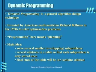
Dynamic Programming History • Bellman. Pioneered the systematic study of dynamic programming inthe 1950s. • Etymology. • Dynamic programming = planning over time. • Secretary of defense was hostile to mathematical research. • Bellman sought an impressive name to avoid confrontation. • "it's impossible to use dynamic in a pejorative sense" • "something not even a Congressman could object to" • Reference: Bellman, R. E. Eye of the Hurricane, An Autobiography.
Algorithmic Paradigms • Greedy. Build up a solution incrementally, myopically optimizing somelocal criterion. • Divide-and-conquer. Break up a problem into two sub-problems, solveeach sub-problem independently, and combine solution to sub-problemsto form solution to original problem. • Dynamic programming. Break up a problem into a series of overlappingsub-problems, and build up solutions to larger and larger sub-problems.
Dynamic Programming Applications • Areas. • Bioinformatics. • Control theory. • Information theory. • Operations research. • Computer science: theory, graphics, AI, systems, ... • Some famous dynamic programming algorithms. • Viterbi for hidden Markov models. • Unix diff for comparing two files. • Smith-Waterman for sequence alignment. • Bellman-Ford for shortest path routing in networks. • Cocke-Kasami-Younger for parsing context free grammars.
0 - 1 Knapsack Problem Knapsack problem. • Given n objects and a "knapsack." • Item i weighs wi > 0 kilograms and has value vi > 0. • Knapsack has capacity of W kilograms. • Goal: fill knapsack so as to maximize total value.
Example • Items 3 and 4 have value 40 • Greedy: repeatedly add item with maximum ratiovi / wi • {5,2,1} achieves only value = 35, not optimal W = 11
Dynamic Programming: False Start • Def. OPT(i) = max profit subset of items 1, …, i. • Case 1: OPT does not select item i. • OPT selects best of { 1, 2, …, i-1 } • Case 2: OPT selects item i. • accepting item i does not immediately imply that we will have toreject other items • without knowing what other items were selected before i, we don'teven know if we have enough room for i • Conclusion. Need more sub-problems!
Adding a New Variable • Def. OPT(i, W) = max profit subset of items 1, …, i with weight limit W. • Case 1: OPT does not select item i. • OPT selects best of { 1, 2, …, i-1 } using weight limit W • Case 2: OPT selects item i. • new weight limit = W – wi • OPT selects best of { 1, 2, …, i–1 } using this new weight limit
Knapsack Problem: Bottom-Up • Knapsack. Fill up an n-by-W array. Input:n, W, w1,…,wn, v1,…,vn for w = 0 to W M[0, w] = 0 fori = 1 to n forw = 1 to W if (wi > w) M[i, w] = M[i-1, w] else M[i, w] = max {M[i-1, w], vi + M[i-1, w-wi ]} returnM[n, W]
Knapsack Algorithm W+1 n+1 OPT = 40
Knapsack Problem: Running Time • Running time.O(n W). • Not polynomial in input size! • "Pseudo-polynomial." • Decision version of Knapsack is NP-complete. • Knapsack approximation algorithm. • There exists a polynomial algorithm that produces a feasible solution that has value within 0.0001% ofoptimum.
Knapsack problem: another DP • Let V be the maximum value of all items, • Clearly OPT <= nV • Def. OPT(i, v) = the smallest weight of a subset items 1, …, i such that its value is exactlyv, If no such item exists it is infinity • Case 1: OPT does not select item i. • OPT selects best of { 1, 2, …, i-1 } with value v • Case 2: OPT selects item i. • new value = v – vi • OPT selects best of { 1, 2, …, i–1 } using this new value
Running time:O(n2V), Since v is in {1,2, ..., nV } • Still not polynomial time, input is: n, logV
Knapsack summary • If all items have the same value, this problem can be solved in polynomial time • If v or w is bounded by polynomial of n, it is also P problem
Longest increasing subsequence • Input: a sequence of numbers a[1..n] • A subsequenceis any subset of these numbers taken in order, of the form and an increasing subsequence is one in which the numbers are getting strictly larger. • Output: The increasing subsequence of greatest length.
Example • Input.5; 2; 8; 6; 3; 6; 9; 7 • Output.2; 3; 6; 9 • 5 2 8636 9 7
directed path • A graph ofall permissible transitions: establish a node ifor each element ai, and add directed edges (i, j)whenever it is possible for ai and aj to be consecutive elements in an increasing subsequence,that is, whenever i < j and ai<aj 6 3 6 9 7 5 2 8
Longest path • Denote L(i) be the length of the longest path ending at i. • for j = 1, 2, ..., n: • L(j) = 1 + max {L(i) : (i, j) is an edge} • return maxj L(j) • O(n2)
How to solve it? • Recursive? No thanks! • Notice that the same subproblems get solved over and over again! L(5) L(1) L(2) L(3) L(4) L(1) L(2) L(3)
Sequence Alignment • How similar are two strings? • ocurrance • occurrence o c u r r a n c e - 6 mismatches,1gap o c c u r r e n c e o c - u r r a n c e 1 mismatch,1gap o c c u r r e n c e o c - u r r - a n c e 0 mismatch, 3gaps - n c e o c c u r r e
Edit Distance • Applications. • Basis for Unix diff. • Speech recognition. • Computational biology. • Edit distance. [Levenshtein 1966, Needleman-Wunsch 1970] • Gap penaltyδ, mismatch penaltyapq • Cost = sum of gap and mismatch penalties.
Sequence Alignment • Goal: Given two strings X = x1 x2 . . . xm and Y = y1 y2 . . . yn findalignment of minimum cost. • Def. An alignment M is a set of ordered pairs xi-yj such that each itemoccurs in at most one pair and no crossings. • Def. The pair xi-yj and xi’ -yj’ cross if i < i', but j > j'.
Cost of M gap mismatch
Example • Ex. X=ocurrance vs. Y= occurrence x1 x2 x3 x4 x5 x6 x7 x8 x9 o c - u r r a n c e o c c u r r e n c e y1 y2 y3 y4 y5 y6 y7 y8 y9 y10
Sequence Alignment: Problem Structure • Def. OPT(i, j) = min cost of aligning strings x1 x2 . . . xi and y1 y2 . . . yj . • Case 1: OPT matches xi - yj. • pay mismatch for xi - yj + min cost of aligning two stringsx1 x2 . . . xi-1and y1 y2 . . . yj-1 • Case 2a: OPT leaves xi unmatched. • pay gap for xi and min cost of aligning x1 x2 . . . xi-1and y1 y2 . . . yj • Case 2b: OPT leaves yj unmatched. • pay gap for yj and min cost of aligning x1 x2 . . . xiand y1 y2 . . . yj-1
Sequence Alignment:Algorithm Sequence-Alignment(m, n, x1 x2 . . . xm, y1 y2 . . . yn,δ,α) { for i = 0 to m M[0, i] = i δ for j = 0 to n M[j, 0] = j δ for i = 1 to m for j = 1 to n M[i, j] = min(α[xi, yj] + M[i-1, j-1],δ+ M[i-1, j],δ+ M[i, j-1]) return M[m, n] }
Analysis • Running time and space. • O(mn) time and space. • English words or sentences: m, n <= 10. • Computational biology: m = n = 100,000. 10 billions ops OK, but 10GB array?
Sequence Alignment in Linear Space • Q. Can we avoid using quadratic space? • Easy. Optimal value in O(m + n) space and O(mn) time. • Compute OPT(i, •) from OPT(i-1, •). • No longer a simple way to recover alignment itself. • Theorem. [Hirschberg 1975] Optimal alignment in O(m + n) space andO(mn) time. • Clever combination of divide-and-conquer and dynamic programming. • Inspired by idea of Savitch from complexity theory.
Space efficient j-1 • Space-Efficient-Alignment (X, Y) • Array B[0..m,0...1] • Initialize B[i,0] = iδ for each i • For j = 1, ..., n • B[0, 1] = j δ • For i = 1, ..., m • B[i, 1] = min {α[xi, yj] + B[i-1, 0],δ + B[i-1, 1],δ + B[i, 0]} • End for • Move column 1 of B to column 0: Update B[i ,0] = B[i, 1] for each i End for % B[i, 1] holds the value of OPT(i, n) for i=1, ...,m
Sequence Alignment: Linear Space • Edit distance graph. • Let f(i, j) be shortest path from (0,0) to (i, j). • Observation: f(i, j) = OPT(i, j).
Sequence Alignment: Linear Space • Edit distance graph. • Let f(i, j) be shortest path from (0,0) to (i, j). • Can compute f (•, j) for any j in O(mn) time and O(m + n) space.
Sequence Alignment: Linear Space • Edit distance graph. • Let g(i, j) be shortest path from (i, j) to (m, n). • Can compute by reversing the edge orientations and inverting theroles of (0, 0) and (m, n)
Sequence Alignment: Linear Space • Edit distance graph. • Let g(i, j) be shortest path from (i, j) to (m, n). • Can compute g(•, j) for any j in O(mn) time and O(m + n) space.
Sequence Alignment: Linear Space • Observation 1. The cost of the shortest path that uses (i, j) isf(i, j) + g(i, j).
Sequence Alignment: Linear Space • Observation 2. let q be an index that minimizes f(q, n/2) + g(q, n/2).Then, the shortest path from (0, 0) to (m, n) uses (q, n/2). • Divide: find index q that minimizes f(q, n/2) + g(q, n/2) using DP. • Align xq and yn/2. • Conquer: recursively compute optimal alignment in each piece.
Divide-&-conquer-alignment (X, Y) • DCA(X, Y) • Let m be the number of symbols in X • Let n be the number of symbols in Y • If m<=2 and n<=2 then • computer the optimal alignment • Call Space-Efficient-Alignment(X,Y[1:n/2]) • Call Space-Efficient-Alignment(X,Y[n/2+1:n]) • Let q be the index minimizing f(q, n/2) + g(q, n/2) • Add (q, n/2) to global list P • DCA(X[1..q], Y[1:n/2]) • DCA(X[q+1:n], Y[n/2+1:n]) • Return P
Running time • Theorem. Let T(m, n) = max running time of algorithm on strings oflength at most m and n. T(m, n) = O(mn log n). Remark. Analysis is not tight because two sub-problems are of size (q, n/2) and (m - q, n/2). In next slide, we save log n factor.
Running time • Theorem. Let T(m, n) = max running time of algorithm on strings oflength m and n. T(m, n) = O(mn). • Pf.(by induction on n) • O(mn) time to compute f( •, n/2) and g ( •, n/2) and find index q. • T(q, n/2) + T(m - q, n/2) time for two recursive calls. • Choose constant c so that:
Running time • Base cases: m = 2 or n = 2. • Inductive hypothesis:T(m, n) ≤2cmn.
Longest Common Subsequence (LCS) • Given two sequences x[1 . . m] and y[1 . . n], finda longest subsequence common to them both. • Example: • x: A B C B D A B • y: B D C A B A • BCBA =LCS(x, y) “a” not “the”
Brute-force LCS algorithm • Check every subsequence of x[1 . . m] to seeif it is also a subsequence of y[1 . . n]. • Analysis • Checking = O(n) time per subsequence. • 2msubsequences of x (each bit-vector oflength m determines a distinct subsequenceof x). • Worst-case running time = O(n2m) = exponential time.
Towards a better algorithm • Simplification: • 1. Look at the length of a longest-commonsubsequence. • 2. Extend the algorithm to find the LCS itself. • Notation: Denote the length of a sequence sby | s |. • Strategy: Consider prefixes of x and y. • Define c[i, j] = | LCS(x[1 . . i], y[1 . . j]) |. • Then, c[m, n] = | LCS(x, y) |.
Recursive formulation • Theorem. • Proof. Case x[i] = y[ j]: • Let z[1 . . k] = LCS(x[1 . . i], y[1 . . j]), where c[i, j]= k. Then, z[k] = x[i], or else z could be extended.Thus, z[1 . . k–1] is CS of x[1 . . i–1] and y[1 . . j–1].
m 1 2 i x : ... j 1 n = y : ...
Proof (continued) • Claim: z[1 . . k–1] = LCS(x[1 . . i–1], y[1 . . j–1]). • Suppose w is a longer CS of x[1 . . i–1] andy[1 . . j–1], that is, |w| > k–1. Then, cut andpaste: w || z[k] (w concatenated with z[k]) is acommon subsequence of x[1 . . i] and y[1 . . j]with |w || z[k]| > k. Contradiction, proving theclaim. • Thus, c[i–1, j–1] = k–1, which implies that c[i, j]= c[i–1, j–1] + 1. • Other cases are similar.
Dynamic-programminghallmark • Optimal substructure • An optimal solution to a problem(instance) contains optimalsolutions to subproblems. • If z = LCS(x, y), then any prefix of z isan LCS of a prefix of x and a prefix of y.
Recursive algorithm for LCS LCS(x, y, i, j) if x[i] = y[ j] then c[i, j] ← LCS(x, y, i–1, j–1) + 1 else c[i, j] ← max{LCS(x, y, i–1, j),LCS(x, y, i, j–1)}

