Lecture 15: Latent Semantic Indexing

1. Prof. Ray Larson University of California, Berkeley School of Information Lecture 15: Latent Semantic Indexing Principles of Information Retrieval

2. Overview • Review • Relevance Feedback • More of Relevance Feedback • Latent Semantic Indexing (LSI)

3. Relevance Feedback in an IR System Storage Line Interest profiles & Queries Documents & data Information Storage and Retrieval System Rules of the game = Rules for subject indexing + Thesaurus (which consists of Lead-In Vocabulary and Indexing Language Formulating query in terms of descriptors Indexing (Descriptive and Subject) Storage of profiles Storage of Documents Store1: Profiles/ Search requests Store2: Document representations Comparison/ Matching Potentially Relevant Documents Selected relevant docs

4. Query Modification • Changing or Expanding a query can lead to better results • Problem: how to reformulate the query? • Thesaurus expansion: • Suggest terms similar to query terms • Relevance feedback: • Suggest terms (and documents) similar to retrieved documents that have been judged to be relevant

5. Relevance Feedback • Main Idea: • Modify existing query based on relevance judgements • Extract terms from relevant documents and add them to the query • and/or re-weight the terms already in the query • Two main approaches: • Automatic (psuedo-relevance feedback) • Users select relevant documents • Users/system select terms from an automatically-generated list

6. Rocchio Method

7. Rocchio/Vector Illustration Information 1.0 D1 Q’ 0.5 Q0 Q” D2 0 0.5 1.0 Retrieval Q0 = retrieval of information = (0.7,0.3) D1 = information science = (0.2,0.8) D2 = retrieval systems = (0.9,0.1) Q’ = ½*Q0+ ½ * D1 = (0.45,0.55) Q” = ½*Q0+ ½ * D2 = (0.80,0.20)

8. Example Rocchio Calculation Relevant docs Non-rel doc Original Query Constants Rocchio Calculation Resulting feedback query

9. Rocchio Method • Rocchio automatically • re-weights terms • adds in new terms (from relevant docs) • have to be careful when using negative terms • Rocchio is not a machine learning algorithm • Most methods perform similarly • results heavily dependent on test collection • Machine learning methods are proving to work better than standard IR approaches like Rocchio

10. Probabilistic Relevance Feedback Document Relevance Given a query term t + - + r n-r n - R-r N-n-R+r N-n R N-R N Document indexing Where N is the number of documents seen Robertson & Sparck Jones

11. Robertson-Spark Jones Weights • Retrospective formulation --

12. Robertson-Sparck Jones Weights Predictive formulation

13. Koenemann and Belkin • Test of user interaction in relevance feedback

14. Relevance Feedback Summary • Iterative query modification can improve precision and recall for a standing query • In at least one study, users were able to make good choices by seeing which terms were suggested for R.F. and selecting among them • So … “more like this” can be useful!

15. Alternative Notions of Relevance Feedback • Find people whose taste is “similar” to yours. Will you like what they like? • Follow a users’ actions in the background. Can this be used to predict what the user will want to see next? • Track what lots of people are doing. Does this implicitly indicate what they think is good and not good?

16. Alternative Notions of Relevance Feedback • Several different criteria to consider: • Implicit vs. Explicit judgements • Individual vs. Group judgements • Standing vs. Dynamic topics • Similarity of the items being judged vs. similarity of the judges themselves

17. Collaborative Filtering (social filtering) • If Pam liked the paper, I’ll like the paper • If you liked Star Wars, you’ll like Independence Day • Rating based on ratings of similar people • Ignores the text, so works on text, sound, pictures etc. • But: Initial users can bias ratings of future users

18. Ringo Collaborative Filtering (Shardanand & Maes 95) • Users rate musical artists from like to dislike • 1 = detest 7 = can’t live without 4 = ambivalent • There is a normal distribution around 4 • However, what matters are the extremes • Nearest Neighbors Strategy: Find similar users and predicted (weighted) average of user ratings • Pearson r algorithm: weight by degree of correlation between user U and user J • 1 means very similar, 0 means no correlation, -1 dissimilar • Works better to compare against the ambivalent rating (4), rather than the individual’s average score

19. Social Filtering • Ignores the content, only looks at who judges things similarly • Works well on data relating to “taste” • something that people are good at predicting about each other too • Does it work for topic? • GroupLens results suggest otherwise (preliminary) • Perhaps for quality assessments • What about for assessing if a document is about a topic?

20. Learning interface agents • Add agents in the UI, delegate tasks to them • Use machine learning to improve performance • learn user behavior, preferences • Useful when: • 1) past behavior is a useful predictor of the future • 2) wide variety of behaviors amongst users • Examples: • mail clerk: sort incoming messages in right mailboxes • calendar manager: automatically schedule meeting times?

21. Advantages • Less work for user and application writer • compare w/ other agent approaches • no user programming • significant a priori domain-specific and user knowledge not required • Adaptive behavior • agent learns user behavior, preferences over time • Model built gradually

22. Consequences of passiveness • Weak heuristics • click through multiple uninteresting pages en route to interestingness • user browses to uninteresting page, heads to nefeli for a coffee • hierarchies tend to get more hits near root • No ability to fine-tune profile or express interest without visiting “appropriate” pages

23. Open issues • How far can passive observation get you? • for what types of applications is passiveness sufficient? • Profiles are maintained internally and used only by the application. some possibilities: • expose to the user (e.g. fine tune profile) ? • expose to other applications (e.g. reinforce belief)? • expose to other users/agents (e.g. collaborative filtering)? • expose to web server (e.g. cnn.com custom news)? • Personalization vs. closed applications • Others?

24. Relevance Feedback on Non-Textual Information • Image Retrieval • Time-series Patterns

25. MARS (Riu et al. 97) Relevance feedback based on image similarity

26. BlobWorld (Carson, et al.)

27. Time Series R.F. (Keogh & Pazzani 98)

28. Using Relevance Feedback • Known to improve results • in TREC-like conditions (no user involved) • So-called “Blind Relevance Feedback” typically uses the Rocchio algorithm with the assumption that the top N documents in an initial retrieval are relevant

29. Blind Feedback • Top 10 new terms taken from top 10 documents • Term selection is based on the classic Robertson/Sparck Jones probabilistic model

30. Blind Feedback in Cheshire II • Perform initial search (using TREC2 Probabilistic Algorithm) next slide

31. TREC2 Algorithm |Qc| is the number of terms in common between the query and the component qtf is the query term frequency ql is the query length (number of tokens) tfiis the term frequency in the component/document cl is the number of terms in the component/document ctfi is the collection term frequency (number of occurrences in collection) Ntis the number of terms in the entire collection

32. Blind Feedback in Cheshire II • Take top N documents and get the term vectors for those documents • Calculate the Robertson/Sparck Jones weights for each term in the vectors • Note that collection stats are used for non-rel documents (i.e. n, n-m, etc)

33. Blind Feedback in Cheshire II • Rank the terms by wtand take the top M terms (ignoring those that occur in less than 3 of the top ranked docs) • For the new query: • Use original freq weight * 0.5 as the weight for old terms • Add wt to the new query length for old terms • Use 0.5 as the weight for new terms and add 0.5 to the query length for each term. • Perform the TREC2 ranking again using the new query with the new weights and length

34. Summary • Relevance feedback is an effective means for user-directed query modification. • Modification can be done with either direct or indirect user input • Modification can be done based on an individual’s or a group’s past input.

35. Today • LSI – Latent Semantic Indexing

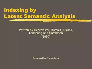
36. LSI Rationale • The words that searchers use to describe the their information needs are often not the same words used by authors to describe the same information. • I.e., index terms and user search terms often do NOT match • Synonymy • Polysemy • Following examples from Deerwester, et al. Indexing by Latent Semantic Analysis. JASIS 41(6), pp. 391-407, 1990

37. LSI Rationale Access Document Retrieval Information Theory Database Indexing Computer REL M D1 x x x x x R D2 x* x x* M D3 x x* x * R M Query: IDF in computer-based information lookup Only matching words are “information” and “computer” D1 is relevant, but has no words in the query…

38. LSI Rationale • Problems of synonyms • If not specified by the user, will miss synonymous terms • Is automatic expansion from a thesaurus useful? • Are the semantics of the terms taken into account? • Is there an underlying semantic model of terms and their usage in the database?

39. LSI Rationale • Statistical techniques such as Factor Analysis have been developed to derive underlying meanings/models from larger collections of observed data • A notion of semantic similarity between terms and documents is central for modelling the patterns of term usage across documents • Researchers began looking at these methods that focus on the proximity of items within a space (as in the vector model)

40. LSI Rationale • Researchers (Deerwester, Dumais, Furnas, Landauer and Harshman) considered models using the following criteria • Adjustable representational richness • Explicit representation of both terms and documents • Computational tractability for large databases

41. LSI Rationale • The only method that satisfied all three criteria was Two-Mode Factor Analysis • This is a generalization of factor analysis based on Singular Value Decomposition (SVD) • Represents both terms and documents as vectors in a space of “choosable dimensionality” • Dot product or cosine between points in the space gives their similarity • An available program could fit the model in O(N2*k3)

42. How LSI Works • Start with a matrix of terms by documents • Analyze the matrix using SVD to derive a particular “latent semantic structure model” • Two-Mode factor analysis, unlike conventional factor analysis, permits an arbitrary rectangular matrix with different entities on the rows and columns • Such as Terms and Documents

43. How LSI Works • The rectangular matrix is decomposed into three other matices of a special form by SVD • The resulting matrices contain “singular vectors” and “singular values” • The matrices show a breakdown of the original relationships into linearly independent components or factors • Many of these components are very small and can be ignored – leading to an approximate model that contains many fewer dimensions

44. How LSI Works • In the reduced model all of the term-term, document-document and term-document similiarities are now approximated by values on the smaller number of dimensions • The result can still be represented geometrically by a spatial configuration in which the dot product or cosine between vectors representing two objects corresponds to their estimated similarity • Typically the original term-document matrix is approximated using 50-100 factors

45. How LSI Works Titles C1: Human machine interface for LAB ABC computer applications C2: A survey of user opinion of computer system responsetime C3: The EPS user interface management system C4: System and human system engineering testing of EPS C5: Relation of user-percieved response time to error measurement M1: The generation of random, binary, unordered trees M2: the intersection graph of paths in trees M3: Graph minors IV: Widths of trees and well-quasi-ordering M4: Graph minors: A survey Italicized words occur and multiple docs and are indexed

46. How LSI Works Terms Documents c1 c2 c3 c4 c5 m1 m2 m3 m4 Human 1 0 0 1 0 0 0 0 0 Interface 1 0 1 0 0 0 0 0 0 Computer 1 1 0 0 0 0 0 0 0 User 0 1 1 0 1 0 0 0 0 System 0 1 1 2 0 0 0 0 0 Response 0 1 0 0 1 0 0 0 0 Time 0 1 0 0 1 0 0 0 0 EPS 0 0 1 1 0 0 0 0 0 Survey 0 1 0 0 0 0 0 0 0 Trees 0 0 0 0 0 1 1 1 0 Graph 0 0 0 0 0 0 1 1 1 Minors 0 0 0 0 0 0 0 1 1

47. How LSI Works 11graph M2(10,11,12) 10 Tree 12 minor C4(1,5,8) C3(2,4,5,8) C1(1,2,3) M1(10) C5(4,6,7) C2(3,4,5,6,7,9) M2(10,11) M4(9,11,12) 2 interface 9 survey 7 time 3 computer 1 human 6 response 5 system 4 user Dimension 2 SVD to 2 dimensions Q(1,3) Blue dots are terms Documents are red squares Blue square is a query Dotted cone is cosine .9 from Query “Human Computer Interaction” -- even docs with no terms in common (c3 and c5) lie within cone. Dimension 1

48. How LSI Works docs X T0 = S0 D0’ terms txd txm mxm mxd X = T0S0D0’ T0 has orthogonal, unit-length columns (T0’ T0 = 1) D0 has orthogonal, unit-length columns (D0’ D0 = 1) S0 is the diagonal matrix of singular values t is the number of rows in X d is the number of columns in X m is the rank of X (<= min(t,d)

49. How LSI Works docs X T ^ = S D’ terms txd txk mxk kxd ^ X = TSD’ T has orthogonal, unit-length columns (T’T = 1) D has orthogonal, unit-length columns (D’D = 1) S0 is the diagonal matrix of singular values t is the number of rows in X d is the number of columns in X m is the rank of X (<= min(t,d) k is the chosen number of dimensions in the reduced model (k <= m)

50. Comparisons in LSI • Comparing two terms • Comparing two documents • Comparing a term and a document