Download
1 / 25
260 likes | 407 Vues
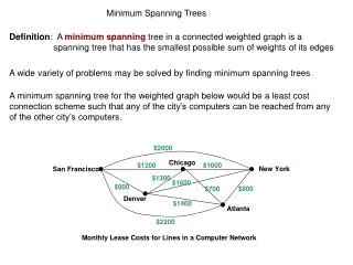
Kedar Dhamdhere Computer Science Department Joint work with: Mohit Singh, R. Ravi (IPCO 05). On Stochastic Minimum Spanning Trees. Outline. Stochastic Optimization Model Related Work Algorithm for Stochastic MST Conclusion. Stochastic optimization.

E N D
Kedar Dhamdhere Computer Science Department Joint work with: Mohit Singh, R. Ravi (IPCO 05) On Stochastic Minimum Spanning Trees
Outline • Stochastic Optimization Model • Related Work • Algorithm for Stochastic MST • Conclusion
Stochastic optimization • Classical optimization assumes deterministic inputs • Real world data has uncertainties • [Dantzig ‘55, Beale ‘61] Modeling data uncertainty as probability distribution over inputs
Common framework [Birge, Louveaux 97] Two-stage stochastic opt. with recourse • Two stages of decision making • Probability dist. governing second stage data and costs • Solution can always be made feasible in second stage
Common framework [Birge, Louveaux 97] Two-stage stochastic opt. with recourse • Two stages of decision making • Probability dist. governing second stage data and costs • Solution can always be made feasible in second stage
Common framework [Birge, Louveaux 97] Two-stage stochastic opt. with recourse • Two stages of decision making • Probability dist. governing second stage data and costs • Solution can always be made feasible in second stage
Stochastic MST Prob = 1/4 Prob = 1/2 Prob = 1/4 Today Tomorrow
Stochastic MST Prob = 1/4 Prob = 1/2 Prob = 1/4 Today’s cost = 2 Tomorrow’s E[cost] = 1
The goal • Approximation algorithm under the scenario model • NP-hardness • Probability distribution given as a set of scenarios
The goal • Approximation algorithm under the scenario model • NP-hardness • Probability distribution given as a set of scenarios
Related work • Stochastic Programming [Birge, Louveaux ’97, Klein Haneveld, van der Vlerk ’99] • Approximation algorithms: Polynomial Scenarios model, several problems using LP rounding, incl. Vertex Cover, Facility Location, Shortest paths [Ravi, Sinha, IPCO ’04]
Related work • Vertex cover and Steiner trees in restricted models studied by [Immorlica, Karger, Minkoff, Mirrokni SODA ’04] • “Black box” model: A general technique of sampling the future scenarios a few times and constructing a first stage solutions for the samples [Gupta et al 04] • Rounding for stochastic Set Cover, FPRAS for #P hard Stochastic Set Cover LPs [Shmoys, Swamy FOCS ’04] • 2-approximation for stochastic covering problem given approximation for the deterministic problem
Our results: approximation algorithm • Theorem: There is an O(log nk)-approximation algorithm for the stochastic MST problem • Hardness: [Flaxman et al 05, Gupta] Stochastic MST is min{log n, log k}-hard to approximate unless P = NP
LP formulation min e c0ex0e+ i pi (e ciexie) s.t. e2 S x0e+ xie¸ 1 8 S ½ V, 1· i· k xie¸ 0 8 e 2 E, 0· i· k Each cut must be covered either in the first stage or in each scenario of the second stage
Algorithm: randomized rounding • Solve the LP formulation • fractional solution: x0e, xie • For O(log nk) rounds • Include an edge independent of others in the first stage solution with probability x0e • Include an edge independent of others in the ith scenario with probability xie
Example Today Tomorrow
Example: round 1 Today Tomorrow
Example: round 1 Today Tomorrow
Example: round 2 Today Tomorrow
Proof idea • Lemma: Cost paid in each round is at most OPT
Proof idea • Lemma: Cost paid in each round is at most OPT • Lemma: In each round, with probability 1/2, the number of connected components in a scenario decrease by 9/10 • At least one edge leaving a component is included with prob 0.63
Proof idea • Lemma: Cost paid in each round is at most OPT • Lemma: In each round, with probability 1/2, the number of connected components in a scenario decrease by 9/10 • At least one edge leaving a component is included with prob 0.63 • After O(log nk) “successful” rounds, only 1 connected component left in each scanario w.h.p.
Other models for second stage costs • Sampling Access: “Black box” available which generates a sample of 2nd stage data O(log n)-approximation in time poly(n,) • : max ratio by which cost of any edge changes • Sample poly(n,) scenarios from “black box”
Other models for second stage costs • Independent costs: second stage cost 2u.a.r [0,1] • Threshold heuristic with performance guarantee OPT + (3)/4 • [Frieze 85] Single stage costs 2u.a.r [0,1]; MST has cost (3) • [Flaxman et al. 05] Both stage costs 2u.a.r [0,1]; Thresholding heuristic gives cost ·(3) – 1/2
Conclusions • Tight approximation algorithm for stochastic MST based on randomized rounding • Extensions to other models for uncertainty in data