Download
1 / 25
490 likes | 1.71k Vues
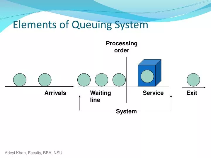
Processing order. Arrivals. Waiting line. Service. Exit. System. Elements of Queuing System. Fantasy Kingdom. Waiting in lines does not add enjoyment Waiting in lines does not generate revenue. Waiting lines are non-value added occurrences. Why is there waiting? Queuing theory

E N D
Processing order Arrivals Waiting line Service Exit System Elements of Queuing System
Fantasy Kingdom Waiting in lines does not add enjoyment Waiting in lines does not generate revenue Waiting lines are non-value added occurrences
Why is there waiting? Queuing theory Mathematical approach to the analysis of waiting lines. Goal of queuing analysis is to minimize the sum of two costs Customer waiting costs Service capacity costs Waiting Lines
Cost to provide waiting space Loss of business Customers leaving Customers refusing to wait Loss of goodwill Quality! Reduction in customer satisfaction Congestion may disrupt other business operations Implications of Waiting Lines
Queuing Analysis- balancing Total Cost = Customer waiting cost + Capacity cost Total cost Cost of service capacity Cost Cost of customers waiting Optimum Service capacity
Population Source Infinite source: customer arrivals are unrestricted Finite source: number of potential customers is limited Number of servers (channels) Arrival and service patterns Variability Arrival/service rate ~ Poisson distribution Inter-arrival/service time ~ negative exponential Queue discipline (order of service) System Characteristics
Poisson distribution • a discrete probability distribution that expresses the probability of a given number of events occurring in a fixed interval of time and/or space if these events occur with a known average rate and independently of the time since the last event. • The expected value of a Poisson-distributed random variable is equal to λ and so is its variance. • P(r) = (e-λ λr ) / r! where • r = arrivals/time unitand • λ = mean arrivals/time unit • f(t) = μe – μt • where t = service timeand • μ = mean service time
Average number on time waiting in line 0 100% System Utilization Performance measures (Operating characteristics) Example 1
Assumptions of queuing systems • Arrivals rate distribution is Poisson with mean of λ • Service times distribution is Negative Exponential with mean = 1/μ (i.e. Service rate distribution is Poisson) • Queue discipline is FIFO • No reneging (customers stay in queue) • No balking • Mean service rate > mean arrival rate (μ > λ) • Calling population is ∞ • Capacity of system is unlimited
Little’s formula • Applicable for all queuing systems at the steady state • L = λ W • Lq = λ Wq • W = 1 / (μ – λ) • Expected time in the system (W) = Expected time in the queue + expected service time. • That is: W = Wq + 1/μ
The M/M/1 queue • Define an interval Δt such that there is • Δt ≤ 1 arrival and Δt ≤ 1 departure. • Probabilities • 1 arrival in Δt = λ Δt • No arrival in Δt = 1 - λ Δt • 1 departure in Δt = μ Δt • No departure in Δt = 1 - μ Δt • 1 arrival and 1 departure = λ Δt . μ Δt = λμ(Δt)2 • No arrival and no departure = (1 - λ Δt)(1 – μ Δt) = 1 - λ Δt - μ Δt + λμ(Δt)2 • Avg. items in the system, L = λ / (μ – λ)
The M/M/1 queue … L = λ / (μ – λ) Wq = λ /(μ (μ – λ)) W = Wq + 1/μ Lq = λ2 / (μ (μ – λ)) P0 = 1 - λ /μ L = Lq + λ /μ
Example • Customers arrive at an ATM machine at an average rate of 20 per hour (assume the arrivals rate is described by a Poisson distribution). The amount of time they spend at the machine takes on average two minutes, but can vary from customer to customer (assume negative exponential distribution). Calculate the average number of customers in the system, the average time they spend in the system, the average number in the queue, the average time spent in the queue and the percentage of the time the machine is idle.
The M/M/s queue (formulae) • Mean effective service rate = sμ • s = # of servers • μ = average service rate per server Assumptions • Must have sμ > λ • Service distributions are the same for all servers.
The M/M/s queue (formulae) P0 = Pn = ( (λ /μ)n / n!) P0 (for n ≤ s) Pn = ( (λ /μ)n / (s! sn-s)) P0 (for n > s) Lq = Po (λ / μ)s ρ / (s! ( 1 - ρ )2 ) where ρ = λ / s μ L = Lq + λ /μ Wq = Lq/ λ W = Wq + 1/μ
Example • A computer room has three printers which can each print an average of five jobs per minute. The average number of jobs entering a single queue for the three machines is twelve per minute. Assuming the queue is M/M/3 calculate the following: • (i) The average time a job is in the system • (ii) The average number of jobs in the system • (iii) Whether any time would be saved for the customers if the three slow printers were replaced by one fast printer, working at 15 jobs per minute.
Single channel, exponential service time Single channel, constant service time Multiple channel, exponential service time Multiple priority service, exponential service time Queuing Models: Infinite-Source Symbols and explanations- Table 18.1 Equations- Table 18.2, 18.3, 18.5 Make sure you understand the context (Read table title)
Processing order 1 3 2 1 1 Arrivals Waiting line Service Exit Arrivals are assigned a priority as they arrive System Priority Model Table 18.5 at P 832 gives you the equations.
Service factor Average number waiting Average waiting time Average number running Average number being served Number in population Finite-Source Formulas
Not waiting or being served Being served Waiting J L H U W T Finite-Source Queuing
Reduce perceived waiting time Magazines in waiting rooms Radio/television In-flight movies Filling out forms Derive benefits from waiting Place impulse items near checkout Advertise other goods/services Other Approaches