Download
1 / 23
230 likes | 388 Vues
Identification of Wiener models using support vector regression. Stefan Tötterman and Hannu Toivonen Process Control Laboratory Åbo Akademi University Finland. Wiener models. Output error identification The dynamic linear part F consist of an orthonormal filter

E N D
Identification of Wiener models using support vector regression Stefan Tötterman and Hannu Toivonen Process Control Laboratory Åbo Akademi University Finland Process Control Laboratory - Åbo Akademi University
Wiener models • Output error identification • The dynamic linear part F consist of an orthonormal filter • The static nonlinear part N consists of a support vector model Process Control Laboratory - Åbo Akademi University
- insensitive loss function y:observation yest: estimated function y y-yest x Process Control Laboratory - Åbo Akademi University
A set of training data: A set of basis functions: Estimation of y is expanded in basis functions Minimization of L and norm of the weight (smoothness, robustness) Support Vector Regression where w is a weight parameter C is a weight Process Control Laboratory - Åbo Akademi University
Support Vector Regression • The optimization problem is transformed to a dual convex optimization problem and the approximation function is given by • Most of the factors (αi - αi’) will be zero, the input vectors corresponding to the nonzero factors forms the so-called support vectors (correspond to observations outside the ε-tube) • K(xi,xj) is the inner-product kernel, commonly RBF Lagrange multipliers Process Control Laboratory - Åbo Akademi University
Support Vector Regression • SVMs can be seen as a network, where all the important network parameters are computed automatically. bias, b K(x,x1) x1 (1-1’) yest K(x,x2) (2-2’) x2 SV Most of the weights (i-’i) will be zero, the other will define the support vectors (m1-m1’) K(x,xm1) xN Input layer RBF with centers x1,...,xm1 Process Control Laboratory - Åbo Akademi University
Some properties of SVR • No need to compute (xi), enough to compute the kernel values directly (kernel trick). • Convex optimization. • Robust algorithm when using L. • Optimal model complexity is obtained automatically as a part of the solution. • Efficient optimization methods exist (high memory requirements). • Hard to involve prior knowledge about the task. • and C must be chosen simultaneously by the user. Process Control Laboratory - Åbo Akademi University
Dynamic linear part • Introducing orthonormal filters to the dynamic linear part have been found useful. • Usually Laguerre or Kautz filter-types are used. • Laguerre filters with a single real-valued pole are well suited for modelling well damped systems. • Kautz filters with a pair of complex-valued poles are suitable for systems which have oscillatory behaviour. Process Control Laboratory - Åbo Akademi University
Dynamic linear part • Laguerre filters q-1 is the backward-shift operator and || 1. Outputs are calculated for k = 1, 2, ..., l where l is the filter order. Process Control Laboratory - Åbo Akademi University
Dynamic linear part • The filter output xk can be derived from the previous filter output xk-1 Process Control Laboratory - Åbo Akademi University
Wiener models • General Wiener model • Wiener model in this identification method Process Control Laboratory - Åbo Akademi University
Identification of Wiener models • Design parameters: • Dynamic linear part: • (filter pole) • l (filter order) • The identified systems dynamics are unknown • Static nonlinear part: • (insensitivity margin) • C (weight) • γ (RBF kernel) Process Control Laboratory - Åbo Akademi University
Example – Control valve model* • The input u(t) is a pneumatic control signal • The output y(t) is a flow through a valve • The simulated model is described by the following equations e(t) is white gaussian measurement noise, standard deviation 0.05 • *T. Wigren, Recursive prediction error identification using the nonlinear Wiener model, Automatica 29(4) (1993) • *A Hagenblad, Aspects of the Identification of Wiener Models, Linköping Studies in Science and Technology, Thesis No. 793, 1999 Process Control Laboratory - Åbo Akademi University
Example – Control valve model • Training data Process Control Laboratory - Åbo Akademi University
Example – Control valve model • Test data Process Control Laboratory - Åbo Akademi University
Example – Control valve model • Laguerre filter of order l = 5 and with the pole = 0.4 was found to be a proper choice • Optimal SVR parameters • γ = 0.1 • = 0.08 • C = 2000 • This choice of parameters results in a model consisting of 146 support vectors • RMSE 0.0541 (train) • RMSE 0.0556 (test) Process Control Laboratory - Åbo Akademi University
Example – Control valve model • Last 100 samples of the test data set Measured output (solid) Model output (dashed) Noisefree output (dotted) Process Control Laboratory - Åbo Akademi University
Example – Control valve model • Output errors (test data) y-ŷ yNF-ŷ Samples Process Control Laboratory - Åbo Akademi University
Example – Control valve model • Laguerre filter parmeter sensitivity table Process Control Laboratory - Åbo Akademi University
Example – Control valve model • SVR parmeter sensitivity table Process Control Laboratory - Åbo Akademi University
Conclusions • This identification method works well for Wiener model identification and gives accurate models • The model is determined by solving a convex quadratic minimization problem (global optimum is always obtained) • Robust performance w.r.t. new data is achieved since SVR is based on structural risk minimization • It is straightforward to extend this method to MIMO systems Process Control Laboratory - Åbo Akademi University