Download

1 / 17
200 likes | 451 Vues
Introduction to Quantum Information Processing QIC 710 / CS 678 / PH 767 / CO 681 / AM 871. Lectures 19–20 (2013). Richard Cleve DC 2117 / QNC 3129 cleve@cs.uwaterloo.ca. Grover ’ s quantum search algorithm. x 1 . x 1 . U f. x n . x n . y . y f ( x 1 ,...,x n ) .

E N D
Introduction to Quantum Information ProcessingQIC 710 / CS 678 / PH 767 / CO 681 / AM 871 Lectures 19–20 (2013) Richard Cleve DC 2117 / QNC 3129 cleve@cs.uwaterloo.ca
x1 x1 Uf xn xn y y f(x1,...,xn) Quantum search problem Given: a black box computing f : {0,1}n {0,1} Goal: determine if f is satisfiable (if x {0,1}n s.t. f(x) = 1) In positive instances, it makes sense to also find such a satisfying assignment x Classically, using probabilistic procedures, order 2n queries are necessary to succeed—even with probability ¾ (say) Grover’s quantum algorithm that makes only O(2n) queries Query: [Grover ’96]
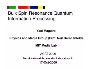
PSPACE NP co-NP 3-CNF-SAT FACTORING P Applications of quantum search The function f could be realized as a 3-CNF formula: Alternatively, the search could be for a certificate for any problem in NP The resulting quantum algorithms appear to be quadratically more efficient than the best classical algorithms known
reflection 2 reflection 1 Prelude to Grover’s algorithm: two reflections = a rotation Consider two lines with intersection angle : 2 2 1 1 Net effect: rotation by angle 2, regardless of starting vector
H X X X H X X X H x1 x1 x1 x1 H U0 Uf xn xn xn xn y y y f(x1,...,xn) y [x=0...0] Grover’s algorithm: description I Basic operations used: Uf x = (1) f(x)x Implementation? U0x = (1)[x=0...0]x Hadamard
iteration 2 ... iteration 1 0 U0 Uf Uf U0 H H H H H 0 Grover’s algorithm: description II • construct state H0...0 • repeatktimes: • apply HU0HUfto state • 3. measure state, to get x{0,1}n, and check if f(x)=1 (The setting of k will be determined later)
Let and A B Grover’s algorithm: analysis I Let A={x{0,1}n : f(x) = 1} and B={x{0,1}n : f(x) = 0} and N= 2n and a=|A| and b=|B| Consider the space spanned by AandB goal is to get close to this state H0...0 Interesting case: a << N
A B Grover’s algorithm: analysis II Algorithm: (HU0HUf)kH0...0 H0...0 Observation: Uf is a reflection about B: UfA =AandUfB =B Question: what is HU0H ? U0 is a reflection about H0...0 Partial proof: HU0HH0...0=HU00...0 =H(0...0) =H0...0
A Since HU0HUf is a composition of two reflections, it is a rotation by 2, wheresin()=a/N a/N More generally, it suffices to set k (/4)N/a B Grover’s algorithm: analysis III Algorithm: (HU0HUf)kH0...0 2 2 2 H0...0 2 When a = 1, we want (2k+1)(1/N) /2 , so k (/4)N Question: what if a is not known in advance?
Unknown number of solutions 1 solution 2 solutions 3 solutions 1 success probability 0 number of iterations 100 solutions 4 solutions 6 solutions success probability very close to zero! √N/2 Choose a randomk in the range to get success probability >0.43
Optimality of Grover’s algorithm
U0 f U1 f U2 f f U3 f Uk |x (1)f(x)|x Assume queries are of the form Optimality of Grover’s algorithm I Theorem: any quantum search algorithm for f: {0,1}n {0,1}must make (2n) queries to f (if f is used as a black-box) Proof (of a slightly simplified version): and that a k-query algorithm is of the form |0...0 where U0, U1, U2, ..., Uk, are arbitrary unitary operations
U0 U0 fr I U1 U1 I fr U2 U2 fr I U3 U3 fr I Uk Uk |0 |0 Optimality of Grover’s algorithm II Define fr: {0,1}n {0,1} as fr (x) = 1 iff x = r Consider |ψr,k versus |ψr,0 We’ll show that, averaging over all r {0,1}n, |||ψr,k |ψr,0|| 2k/2n
|ψr,i U0 I U1 I U2 fr U3 fr Uk i ki |0 Note that |ψr,k |ψr,0 =(|ψr,k |ψr,k1)+ (|ψr,k1 |ψr,k2)+ ... +(|ψr,1 |ψr,0) which implies |||ψr,k |ψr,0|| |||ψr,k |ψr,k1|| + ... + |||ψr,1 |ψr,0|| Optimality of Grover’s algorithm III Consider
query i query i+1 |ψr,i query i query i+1 U0 U0 I I U1 U1 I I U2 U2 I fr U3 U3 fr fr Uk Uk |ψr,i-1 |0 |0 Therefore, |||ψr,k |ψr,0|| Optimality of Grover’s algorithm IV |||ψr,i |ψr,i-1|| =|2i,r|,since query only negates|r
Optimality of Grover’s algorithm V Now, averaging over all r {0,1}n, (By Cauchy-Schwarz) Therefore, for somer{0,1}n, the number of queries k must be (2n), in order to distinguish fr from the all-zero function This completes the proof