Download
1 / 24
240 likes | 247 Vues
This tutorial provides a step-by-step workflow for processing marine geometry data and creating fold maps from seismic data. It also includes a suggested workflow for deriving a Claritas .3dgrid file. Examples for using JCS for multi-line 2D or 3D processing are also provided.

E N D
Introduction This 3D MARINE GEOMETRY tutorial is provided as a production workflow from reformat through to creation of fold maps from the seismic data. The presentation also details a suggested workflow for deriving a Claritas .3dgrid file for use with the BIN3D module. The tutorial also provides useful examples for how to use JCS to industrialise Claritas job flows for multi line 2D or 3D.
Input Dataset Data supplied are single sample Claritas internal format datasets after reformat from SegD. Six datasets are included, and contain all 61 saillines as concatenated onto LTO tapes. Shotpoint Interval : 25 Metre Flip-Flop Group Interval : 12.5 Metres Number of Channels : 6x240 Cable Length : 3000 Metres Data Length : 2ms Sample Rate : 2ms
How to Restore a Claritas Archive file GLOBE Claritas tutorials are generally supplied as self contained project archives, created by the Archive option under the Projects tab on the launcher. To restore a GLOBE Claritas archive (*.ca) select the Restore option on the Projects tab. The following are the key parameters from the form:- The Input archive filename parameter defines where to read the *.ca file from. The Parent directory for projects parameter defines where you wish to output the restored project to. The Project name parameter allows you to define the name to save the project as. The Data directory parameter allows you to optionally define a disk area for the seismic data only.
Job 00 - Reformat The Initial job flows for the supplied production processing sequence cover reading data files from tape and reformatting them from standard SegD format to Claritas internal format. This has already been done for the supplied data which are single sample Claritas internal format datasets The following additional processing is applied in jobs READSEGD_0x.job. • Data is truncated to 1 sample. • Key headers MIN/MAX values are listed using the RANGE module. The QC job (JOB00_TRPRINT_x.job) then lists key headers for channel 1 on every shotid. • The SHOTID header has been renumbered sequentially from 1 for all shots on each tape. This enables extraction of individual saillines from concatenated datasets.
Defining a 3D GRID file In this example we will take four corner points for the survey from the P190 navigation files for the HB3D survey. For new acquisition you can use the pre-plot map to pick a suitable origin and inline azimuth. These corner points should then be plotted on an excel spreadsheet (or open office equivalent etc). Then using the plot, define a suitable origin point and angle in degrees (or use the Sailline acquisition azimuth as a suitable approximation). On the HB3D survey acquisition azimuth’s of 28 and 208 Degrees were used, we will use an azimuth of 28 degrees with an origin at the bottom right corner of the survey
3D GRID Definition Utility Using the ‘Set up 3D grid’ parameter form input your calculated Origin and Inline Azimuth, the Crossline Azimuth is automatically calculated. Define the desired IL/XL spacing and Min/Max IL/XL’s. Select Left or Right handed grid – A grid is left handed if when standing on the first XL of an IL and looking down the inline in the increasing XL direction, increasing IL’s are on your left hand side. INLINE_CDP parameter defines how the Claritas 3D CDP number can be broken down into its constituent IL & XL numbers. Typically INLINE_CDP = 10000
3D GRID Definition Utility The new 3D Grid definition tool now enables you to confirm that the grid is suitable by allowing the user to input either IL/XL pairs or XY coordinate pairs and have the application return the resulting IL/XL or XY coordinate. This will allow you to check that your origin is suitable for the entire survey as you can check that the data sits inside the defined grid and returns valid IL or XL numbers.
Job01 – Nav-Seis merge and Binning. The initial job flow reads in datasets output from READSEGD, selects data volumes related to particular SAILLINES, and creates desired headers such as Line_SEQ, SAILLINE and Gun Mask etc. The NAVHDR module is required in the job flow as this creates some key headers which are used by ADDP190. These are as follows:- • SAILLINE : 16 Character line name i.e. 1630P1-001, 1630R1-005 1630I1-010, supports alphanumeric character strings. • LINE_SEQ : Acquisition sequence number ie 001, 005 or 010. • SEISTIME : Time of shot from the Acquisition system in Julian seconds derived from day, hour, minute, second seismic trace headers. • SEISGUN : Gun-code if available taken from seismic trace header. • NAVTIME : Time of shot from the navigation P1/90 files, also in Julian seconds.
Job01 – Nav-Seis merge and Binning. • NAVGUN : Gun-code taken from navigation P1/90 files. • NAVSPT : Shot point taken from navigation P1/90 files. • CABLENO : Cable-number from P1/90 files. • CABLETR : Sequential trace count within the cable/channelset. • GUNCABLE : Concatenation of seisgun and cablenumber in order that unique 2D sailline profiles can be extracted from any 3D sailline. The created SAILLINE/LINE_SEQ headers are used to match the correct navigation data to the supplied seismic line. SEISTIME along with SHOTID are used when merging navigation into the seismic trace header on a shot by shot basis or confirm the validity of the data merge, along with SEISGUN. The additional headers CABLENO, CABLETR and GUNCABLE are used to apply processes to individual 2D shot gathers, or for QC purposes.
Job01 – Nav-Seis merge and Binning. ADDP190 requires a *.sfl list file containing input P190 datasets and creates a *.navline file which lists SAILLINES, MIN/MAX SHOTID and NAVTIME for the lines encompassed by the supplied P190 files. Navigation can be merged with seismic data based on shotpoint or timestamp. The quality of the merge can be checked based on Shotpoint, Time, Shotpoint & Guncode (Mask) and Time & Guncode.
Job01 – Nav-Seis merge and Binning. As well as writing the Shot and Receiver XY coordinates into the trace headers ADDP190 can also create a unique SP number which is a concatenation of the SHOTID header and the Line Sequence number, this can be written to a user specified header word to create a unique SP number. The ADDP190 module can also outputs *.sht and *.txy files which contain source position and receiver position XY coords. This information, if required, can be input into the GLOBE Claritas Geometry application in order to generate a fold map from navigation rather than seismic data.
Job01 – Nav-Seis merge and Binning. The following headers are created or updated by ADDP190:- Always updated :- • SOURCE_X SOURCE_Y REC_X REC_Y OFFSET SOURCE_WATER Additionally the following extended trace headers can also be updated if required:- • D_LON D_LAT D_SRC_X D_SRC_Y D_REC_X D_REC_Y F_OFFSET F_WATERDEP F_CABLEDEP VESSELID TAILBUOYID NAVTIME NAVGUN CABLENO CABLETR GUNCABLE The headers pre-fixed ‘D_’ are double precision integer format, and those pre-fixed ‘F_‘ are floating point format headers.
Job01 – Nav-Seis merge and Binning. The BIN3D module uses the previously created 3dgrid definition to bin the supplied traces based on the Source and Receiver XY coordinates. The 3D CDP Grid can be supplied in the form of a *.3dgrid file, as previously covered, or as a GLOBE Claritas *.geom file from the geometry application. The module writes the following seismic trace headers:- CDP INLINE CROSSLINE CDPTRACE CDP-X CDP-Y
Job01 – Nav-Seis merge and Binning. BIN3D also has the capability to create the following dynamic trace headers if required:- GC_SOURCE_X GC_SOURCE_Y GC_REC_X GC_REC_Y GC_CDP_X GC_CDP_Y These will contain the rotated grid coordinates of the source, receiver and CDP bin centres in IEEE4 format.
Job02 – Partial Stack. Once the data has been binned and navigation applied to the headers we then move onto stacking the data in order to create fold maps and other QC’s. The initial job reads the output from JOB01 and performs a partial stack on a sailline by sailline basis. The HORI_SUM header contains the stack fold for each CDP on output, with the stack scalar also optionally preserved in the STACK_LIVE dynamic trace header.
Job02 – Full Volume Stack. Run the Job02_partial_stack_concat.job to combine all output datasets from the J0B02_PARTIAL_STACK jobs into a single dataset. Using SEISREAD read & sort the concatenated dataset. Then using the various HEADER manipulation capabilities available generate the desired headers which will be used to generate the Fold and other QC maps required. The output dataset is then used as input for the JOB02_FV_AREAL.job. This job outputs QC displays which allow the user to check the stack fold, and where holes exist try and correlate these with the SAILLINE/LINE_SEQ’s processed.
Producing a Fold map from the P190 data If required you can generate a Fold Map from the UKOOA P1/90 data. Initially the raw P1/90 files need to be reformatted to inputs suitable for the Geometry applications. This can be done using either the P190->SHTTXY utility, or using the outputs from ADDP190 which also generate .SHT and .TXY files. The individual SHT and TXY files need to be merged which can be done using the UNIX cat command.
P190->SHTTXY utility. Only mandatory parameters are for Input and Output datasets. I would recommend defining the no of Channels and supplying a multiplier for the Sequence number. The Sequence Number multilpier defines how a unique SP number is defined, particularly useful for 3D surveys where each Sailline will have similar SP numbers.
Geometry Application Initial input to the geometry application is the concatenated *.sht file. On input you are likely to be asked if you would like to sort the .sht file, if yes a new *.sht file will be created and saved to the GEOMETRY partition of the project. Sorting may provide faster input if you reload the data later on. Then select create 3D geometry database from the Make menu, this reads in the .txy file associated with the original input .sht file.
Geometry Application - Continued Before creating 3D CDP gathers, you must first define your 3D bin grid using the specify 3D grid option from the HITPOINTS menu. The applicable options are to a) define based on Origin and IL/XL azimuth (in degrees), or b) based on Origin and IL/XL coordinates. The HITPOINTS (Grid) can then be plotted on the Geometry Applications Map grid to confirm its suitability. Once you are happy with your grid definition you can move onto the next step in the Geometry process.
Geometry Application - Continued From the MAKE drop down menu select 3D CDP Gather, and parameterise the pop up form as required for your dataset, correctly defining inline/crossline increments in metres. Once you have accepted the parameters the application goes off and bins the data according to your supplied grid and parameters. When the binning process is complete a pop up diagnostic window will appear providing first level QC of the binning process. Allowing you to identify where the binning process maybe compromised. Further interactive QC can be carried out using the different display options for the Map interface.
Comments All Master job decks and JCS files are provided for this tutorial, suggested workflows for deriving the 3dgrid files are our preferred methodologies, you may develop or have your own workflows. When you have finished working through the tutorials you should have produced a fold map for the HB3D survey. The tutorial should also supply you with robust example workflows you would need to generate fold map for your own projects.