Download
1 / 56
560 likes | 663 Vues
Supervised Rule Induction for Relational Data. Mahmut Uludağ Supervisor: Prof. Dr. Mehmet R. Tolun Ph.D. Jury Presentation Eastern Mediterranean University Computer Engineering Department February 25, 2005. Outline. Introduction ILA and ILA-2 algorithms Overview of the RILA system

E N D
Supervised Rule Inductionfor Relational Data Mahmut Uludağ Supervisor: Prof. Dr. Mehmet R. Tolun Ph.D. Jury Presentation Eastern Mediterranean University Computer Engineering Department February 25, 2005
Outline • Introduction • ILA and ILA-2 algorithms • Overview of the RILA system • Query generation • Optimistic estimate pruning • Rule selection strategies • Experiments and results • Conclusion
Motivation for relational data mining • Traditional work in statistics and knowledge discovery assume data instances form a single table • Not always practical to represent complex objects in one single table • RDBMS are widely used • Efficient management of data • Indexing and query services, transaction and security support • Can store complex data • Data mining without transferring to a new location Cites Author Paper
Previous work – ILP based algorithms • Prolog is the main language to represent objects and relations between the objects • Incremental learning, incorporation of background knowledge • Initial research: deterministic rules • Recent research: statistical learning • Main obstacle to widespread acceptance; dependency on a Prolog server
DMax; a modern ILP based data mining system • Client-server architecture; java client, ILProlog server Example output rule: Source: www.pharmadm.com
child parent toy age>30 Previous work – relational data mining framework • (Knobbe et al, 1999) • Client – server architecture • Selection graphs • Algorithm to translate selection graphs into SQL • MRDTL and MRDTL-2 algorithms, Iowa State University • M.Sc. Study in METU, Serkan Toprak, 2004
Previous work – graph mining • Typical inputs are labelled graphs • Efficient tools in describing objects and the way they are connected • Subgraph isomorphism • Scalability problems • Avoid loading complete graph data into the main memory; partitioning • Nearly equivalent formalisms: • Graphs ≈ Database tables ≈ Prolog statements
ILA • Levelwise search • construct hypotheses in the order of the increasing number of conditions (i.e. at first, building hypotheses with one condition, then building hypotheses with two conditions, and so on) • Finds the smallest and completely accurate rule set that represents the training data
ILA-2 • Noise-tolerant evaluation function • score(hypothesis) = tp - pf * fn • tp is the number of true positive examples • fn is the number of false negative examples • pf stands for penalty factor, a user-defined minimum for the proportion of tp to fn • not sensitive to distribution of false values • Multiple rule selection after a learning loop redundant rules • Implemented by modifying the source code of the C4.5 algorithm; some features inherited from C4.5
RILA • What is new when compared to ILA and ILA-2 • Architecture • Performance • Internal representation of rules • Construction of hypotheses
RILA – what is new • Select late rule selection strategy; as an alternative to the select early strategy • An efficient implementation • hypotheses can be refined by adding new conditions, they do not need to be generated from scratch in each learning loop • Optimistic estimate pruning (beam search) • Normalized hypotheses evaluation function
Architecture of the system Discovery system SQL, meta data queries Hypotheses DBMS JDBC driver Rules Result sets, meta data • Traversing relational schema • Hypothesis construction • Conversions to SQL • Rule selection • Pruning
How tables are visited? Junction table First level – stops in the junction table? Extension levels – extends complex hypotheses only by using attributes from the other side of the junction relation Interaction Target table Gene Composition • Example hypotheses that can be generated: • If a gene has a relation r then its class is c • If a gene has a property p and relation r then its class is c • If a gene has a relation r to a gene having property p then its class is c
Internal representation of an example rule Interaction Composition Composition Conditions: Class=‘Nucleases’ type=‘Genetic’ Complex=‘Intracellular transport’ composition1.id=gene1.id interaction.id1=gene1.id composition2.id=gene2.id Gene Gene Gene Localization=‘extracellular…’ Localization=‘extracellular…’ interaction.id2=gene2.id IF gene1.Composition.Class = ‘Nucleases’ AND Interaction.Type = ‘Genetic’ AND gene2.Composition.Complex = ‘ Intracellular transport’ THEN gene1.Localization = extracellular… gene1.id=interaction.id1 Gene Localization=‘extracellular…’
Query generation • SQL template for building size one hypotheses • Numeric attributes • Refinement of hypotheses • How a hypothesis is represented in SQL? • How a hypothesis is extended by a condition from the other side of an many-to-many relation?
SQL template for building size one hypotheses Select attr, count(distinct targetTable.pk)from covered, path.getTable_list()where path.getJoins() andtargetTable.classAttr = currentClass and covered.id = targetTable.pk and covered.mark=0group by attr
Numeric attributes • Discretization results are stored in a temporary table • Columns: table_name, attribute_name, interval_name, min_value, max_value disc.table_name = ‘table’ anddisc.attribute_name = ‘attr’ andattr > disc.min_val andattr < disc.max_val SQL:
Refinement of hypotheses Select attr, count(distinct targetTable.pk)from covered, table_list, hypothesis.table_list()where targetAttr= currentClass andjoin_list andhypothesis.join_list() covered.id = targetTable.pk and covered.mark=0group by attr;
How a hypothesis is extended by a condition from the other side of a many-to-many relation? Select GENE_B.CHROMOSOME, count (distinct GENE.GENEID) from COMPOSITION, GENE, GENE GENE_B, INTERACTION where INTERACTION.GENEID2=GENE_B.GENEID and INTERACTION.GENEID1=GENE.GENEID andINTERACTION.EXPR > 0.026 andINTERACTION.EXPR < 0.513 and COMPOSITION.PHENOTYPE = 'Auxotrophies' and COMPOSITION.GENEID=GENE.GENEID andGENE.LOCALIZATION = 'ER'group by GENE_B.CHROMOSOME
Optimistic estimate pruning • Avoid working on hypotheses which are unlikely to result in satisfactory rules • F-measure criteria to assess hypotheses • 2 * recall * precision / ( recall + precision ) • Two types of pruning • Extend only n best hypotheses (beam search) • Minimum required f value in order a hypothesis to take place in the hypothesis pool (similar to minimum support pruning)
Rule selection strategies • Select early strategy • Why do we need another strategy? • Select late strategy
Learning algorithm when using the select early strategy size=1 If size is 1 then build initial hypotheses otherwise extend current hypotheses select p rule(s) yes size is smaller than m? any rules selected? no, size++ yes no mark covered objects all examples covered? no yes end
Example training data to demonstrate the case where the select late strategy performs better than the select early strategy
Learning algorithm when using the select late strategy start Build initial hypothesis set Extend hypothesis set size < max size? Select Rules no yes, size++ end
Rule selection algorithm when using the select late strategy start Select hypothesiswith the highest score Is the score positive? no yes - Mark examples covered by this hypothesis - If no positive examples covered then return - Recalculate the score using the effective cover - If the new score is higher than the score of the next hypothesis or score of the hypothesis was previously reduced more than lthen assert the hypothesis as a new rule otherwise undo markings and set the score to the new score calculated all examples covered? yes no end
Experiments • Summary of the parameters • The genes data set • The mutagenesis data set
Summary of the parameters • Parameters applicable both to the select late and to the select early strategies • pf is a user-defined minimum for the proportion of the true positives to the false negatives • m is the maximum size for hypotheses • Parameter applicable only for the select early strategy • p is the maximum number of hypotheses that can be selected as new rules after a search iteration • Parameter applicable only for the select late strategy • l is the limit on rule selection recursion • Optimistic estimate pruning parameters • f is the minimum acceptable F-measure value • n is maximum number of hypotheses that can be extended in each level during the candidate rules generation phase of the mining processes
The ‘genes’ dataset of KDD Cup 2001 COMPOSITION INTERACTION GENE GENEID1 GENEID GENEID GENEID2 Essential Class Type Chromosome Complex Expression Phenotype Localization Motif 910 rows Function Junction table Many-to-many relation between genes 862 rows 4346 rows
Test results for the localization attribute using the select early strategy, pf=2, m=3
Test results for the localization attribute using the select late strategy pf=2, m=3, l=0, f=0.01
Test results for the localization attribute using the select late strategy pf=2, m=3, l=100, f=0.01
Why we did not have better results on the genes data set? • Cup winner’s accuracy 72.1% • MRDTL 76.1% accuracy • Serkan 59.5% accuracy • rila best accuracy 85.8% with 60.9% coverage • rila best coverage 65.3% with 81.5% accuracy • Missing values? no • Default class selection? no • Deteriorated performance when the number of class values is high • Distribution of false values among classes not taken into account • Problem when number of examples in different classes are not evenly distributed
Schema of the mutagenesis database BOND ATOM MOLECULE ATOM_ID1 Molecule_id ATOM_ID ATOM_ID2 Log_mut Molecule_id Type Logp Element Lugmo Type Ind1 Charge Inda Label
Cross validation test results using the select early strategy on the mutagenesis data for different p* values *maximum number of rules selected when each time the rule selection step is executed
Cross validation test results using the select early strategy and OEP on the mutagenesis data for different n values
Cross validation test results using the select late strategy on the mutagenesis data p =1, f=0.01, l=0
Cross validation test results using the select late strategy on the mutagenesis data p =1, f=0.01, l=10
Cross validation test results using the select late strategy on the mutagenesis data p =1, f=0.01, l=100
Comparison to others results on mutagenesis data • The best results by RILA (Table 2 and Table 5) • accuracy 98.26% • coverage 91.49% • The best results reported in (Atramentov et al. 2003) • accuracy 87.5% • The best results reported by the originators (King et al. 1996) of the data set • accuracy 89.4%, (number of correct predictions divided by the number of predictions)
Conclusion • A new relational rule learning algorithm has been developed with two different rule selection strategies • Several techniques used to have reasonable performance; refinement of hypotheses, pruning • The results on the mutagenesis data are better than other results cited in the literature • Compared to traditional algorithms, there is no need to move relational data to another location; scalability, practicality • Techniques employed can be used to develop relational versions of other traditional learning algorithms
FOIL, a set-covering approach • [Cameron Jonaes and Quinlan 1994] • Begins with the most general theory • Repeatedly adds a clause to the theory that covers some of the positive examples and few negative examples • Covered examples are removed • Continue until the theory covers all positive examples
Previous work – unsupervised algorithms • WARMR [Dehaspe et al., 1998] finds relational association rules (query extensions) • Input – Prolog database • Specification in the WARMODE language, limits the format of possible query extensions • SUBDUE [Cook and Holder, 1994] discovers substructures in a graph • Output – the substructure selected at each iteration as the best to compress the graph • PRM [Getoor et al., 2002] reinterpret Bayesian networks in a relational setting • Captures the probabilistic dependence between the attributes of interrelated objects • Link analysis • Models generated by some unsupervised learning algorithms can be used for prediction tasks; WARMR, PRM, not SUBDUE
Relational rule induction • Schema graph represents structure of the data • tables = nodes • foreign keys = edges • Multiple tables can represent several objects and relations between the objects • Users should select tables that represent the objects they are interested in
An example relational rule Composition IF Composition.Class = ‘ATPases’ AND Composition.Complex = ‘ Intracellular transport’ THEN Gene.Localization = extracellular.. Gene
Many-to-many relations Junction table • Junction tables • Between different classes • Between objects of the same class • Recursive queries are needed to extract data between different classes Junction table between objects of the same class
Example rule having a many-to-many relation Composition IF gene1.Composition.Class = ‘Nucleases’ AND Interaction.Type = ‘Genetic’ AND gene2.Composition.Complex = ‘ Intracellular transport’ THEN gene1.Localization = extracellular… Interaction Gene
Performance • Dynamic programming • refinement of hypotheses • Pruning • Minimum support pruning • Optimistic estimate pruning • Avoid redundant hypotheses • Smart data structures
Tabular representation of the links in the example rule IF gene1.Composition.Class = ‘Nucleases’ AND Interaction.Type = ‘Genetic’ AND gene2.Composition.Complex = ‘ Intracellular transport’ THEN gene1.Localization = extracellular…
Building size one hypotheses Vector buildSizeOneHypotheses(String class, String table name, Path path){ For each column in the selected table { If ( column is not the target attribute and not a primary key and not a foreign key) { Check whether the table is the target table Check whether the column is numeric Select the proper SQL template and generate SQL(path) result set = execute generated SQL hypotheses += generated hypotheses using the result set } } For each table linked by a foreign key relation{ If the linked table was not visited before(check the path) hypotheses += buildSizeOneHypotheses(class, linked table name, updated path) } return the hypotheses }