Download
1 / 44
450 likes | 789 Vues
Valence Bond And Molecular Orbital Theories Overview. Parts of the material in today’s lecture have been borrowed from the web site of Professor Peter M. Hierl of the University of Kansas. Rationalization within the VB model: “Promote” a 2s electron. C 2s 1 2p x 1 2p y 1 2p z 1.

E N D
Valence Bond And Molecular Orbital Theories Overview Parts of the material in today’s lecture have been borrowed from the web site of Professor Peter M. Hierlof the University of Kansas
Rationalization within the VB model: “Promote” a 2s electron C 2s1 2px1 2py1 2pz1 Origins of Hybridized Orbitals: Promotion of an electron to a higher energy level C ground state: 2s2 2px1 2py1 Suggests only 2 bonds possible -we know C normally exhibits 4 bonds
Such schemes of electron promotion have been formulated to produce hybrid orbitals that account for the known molecular geometries 2s1 2px1 sp 2s1 2px1 2py1 sp2 2s1 2px1 2py1 2pz1 sp3 Note: You can mix and match – i.e. an sp2 orbital and a p orbital are often invoked to describe bonds in C compounds
The resultant orbital has four large lobes pointed at the corners of a tetrahedron Hybrid orbitals are formed by the linear combination of other atomic orbitals, For the sp3 hybrid orbital: h1 = s + px + py + pz h2 = s - px - py + pz h3 = s - px + py - pz h4 = s + px - py - pz
Another Model: Molecular Orbital Theory MO Theory Universally accepted for modeling bonding in inorganic and organic chemistry
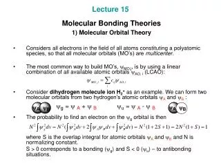
The model assumes that the wavefunction for the N electrons in a molecule is product of N one-electron wavefunctions = (1) (2) (3) …. (N) The one-electron wavefunctions (x) are the MOLECULAR ORBITALS The square of the wavefunction gives the probability distribution for the electron in the molecule
Molecular orbitals are modeled as superimpositions of the individual atomic orbitals in a molecule Linear Combination of Atomic Orbitals LCAO LCAO = sum with weighting coefficients For hydrogen molecule: = cAA + cBB • = hydrogen A.O C = coefficient -relative contribution from each H
The linear combination giving the lowest energy for H2 has cA2 = cB2 cA = cB = 1 • Orbitals with two lowest energy levels: • + = cAA + cBB • - = cAA - cBB Constructive interference Destructive Interference
Antibonding Orbital Bonding Orbital The enhancement of e- density in the internuclear region arising from constructive interference The destructive interference leading to a nodal surface in an antibonding orbital
Molecular orbital energy level diagram For the H2 molecule Origin of the importance of the electron pair bond The size of the energy gap can be determined by determining spectroscopic absorptions due to electronic transitions (Photoelectron spectroscopy) Pauli exclusion principle: ONLY 2 ELECTRONS PERLEVEL (spin paired)
Photoelectron Spectra: Read on your own Heteronuclear Diatomics: Read on your own Bond Properties in the MO Model Bond Order: An electron pair in a bonding orbital = +1 An electron pair in an antibonding orbital = -1 b = ½ (n – n*) n = number of electrons in bonding orbitals n* = number of electrons in antibonding orbitals
+ + + - g u + - + - + - - + u g MO Energy Level Diagram For N2 b = ½ (2 + 4 + 2 – 2) = 3
Bond Strength correlates with Bond Order HB = +946 kJ/mol for nitrogen
Bond Correlations Bond Strength Bond Length Bond Enthalpy increases as B.O. increases Bond Length decreases as B.O. increases
Correlation of bond strength with bond length
Molecular Orbital Theory Remember that the closer to AO’s of appropriate symmetry are in energy, the more they interact with one another and the more stable the bonding MO that will be formed. This means that as the difference in electronegativity between two atoms increases, the stabilization provided by covalent bonding decreases (and the polarity of the bond increases). If the difference in energy of the orbitals is sufficiently large, then covalent bonding will not stabilize the interaction of the atoms. In that situation, the less electronegative atom will lose an electron to the more electronegative atom and two ions will be formed. AO(1) AO(1) AO(1) AO(1) AO(2) AO(2) AO(2) AO(2) Most covalent Polar Covalent Ionic DX < 0.5 : covalent 2 > DX > 0.5 : polar DX > 2 : ionic
MO’s for Polyatomic Molecules Linear trihydrogen MO for trihydrogen: linear combination of AO’s on 3 H HA, HB, HC: 1sA, 1sB, 1sC 1 = 1sA + 1sB + 1sC Lowest energy MO; bonding between all H
Three MO’s of trihydrogen 3 = 1sA – 21/21sB + 1sC Antibonding orbital 2 = 1sA - 1sC Non-bonding orbital
In General: A few rules: • More nodes more antibonding, higher energy • Non-nearest neighbour interactions • weakly bonding if orbital nodes of same sign • weakly antibonding if different signs • Orbitals constructed from lower energy AO’s have • lower energy (s orbitals produce lower energy MO’s • than p orbitals) From N atomic orbitals, can construct N molecular orbitals
12 electrons all accommodated in bonding or nonbonding orbitals. No antibonding orbitals occupied. MO energy level diagram for hypervalent SF6
Molecular Orbital Theory “Infinite” polyatomic molecules An adaptation of MO theory is also used to treat extended (essentially infinite) “molecular” systems such as pieces of a metal (or an alloy) or a molecule such as a diamond. Remember that whenever atomic orbitals have appropriate symmetry and energy, they will interact to form bonding and anti-bonding MO’s. We have only considered small molecules but there are essentially no limits to the number of atoms that can mix their corresponding AO’s together. This mixing must occur because of the Pauli exclusion principle (i.e. so that no two electrons in the solid have the same quantum numbers). MO As the number of interacting atoms (N) increases, the new bonding or anti-bonding MO’s get closer in energy. anti-bonding AO(1) AO(2) bonding In the extreme, the MO’s of a given type become so close in energy that they approximate a continuum of energy levels. Such sets of MO’s are known as bands. In any given band, the most stable MO’s have the most amount of bonding character and the highest energy MO’s are the most anti-bonding. The energy difference between adjacent bands is called the band gap.
Valence Bond Theory Separate atoms are brought together to form molecules. The electrons in the molecule pair to accumulate density in the internuclear region. The accumulated electron density “holds” the molecule together. Electrons are localized (belong to specific bonds). Basis of Lewis structures, resonance, and hybridization. Very poor theory for obtaining quantitative bond dissocation energies. Good theory for predicting molecular structure. Molecular orbital theory Molecular orbitals are formed by the overlap and interaction of atomic orbitals. Electrons then fill the molecular orbitals according to the aufbau principle. Electrons are delocalized (don’t belong to particular bonds, but are spread throughout the molecule). Can give accurate bond dissociation energies if the model combines enough atomic orbitals to form molecular orbitals. Model is complex and requires powerful computers for even simple molecules. MO and VB compared