Download
1 / 16
160 likes | 227 Vues
Acoustic Rapid Environmental Assessment. Possible SVP realizations. Ensemble of HOPS/ESSE forecasts. Current Time. Future Time. Sensing. Ocean-Acoustic Modeling and Predictions. In-situ measurement data. Optimization & Control. Ocean and acoustic forecasts & uncertainties.

E N D
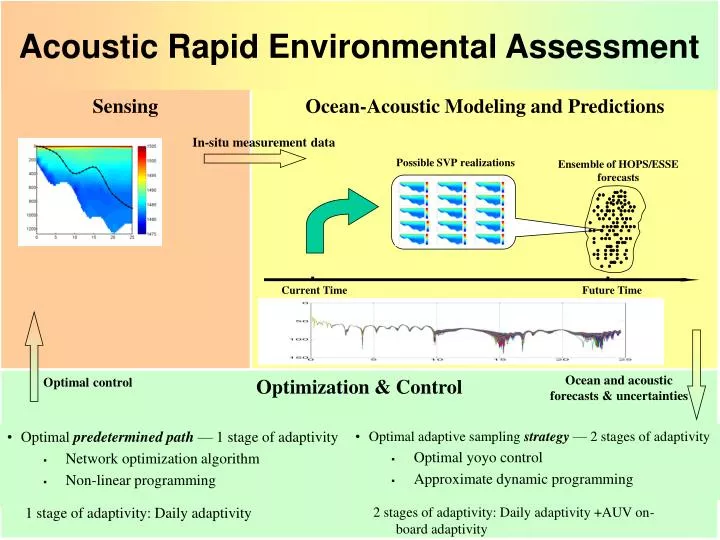
Acoustic Rapid Environmental Assessment Possible SVP realizations Ensemble of HOPS/ESSE forecasts Current Time Future Time Sensing Ocean-Acoustic Modeling and Predictions In-situ measurement data Optimization & Control Ocean and acoustic forecasts & uncertainties Optimal control • Optimal predetermined path— 1 stage of adaptivity • Network optimization algorithm • Non-linear programming • Optimal adaptive sampling strategy — 2 stages of adaptivity • Optimal yoyo control • Approximate dynamic programming 1 stage of adaptivity: Daily adaptivity 2 stages of adaptivity: Daily adaptivity +AUV on-board adaptivity
Adaptive Rapid Environmental Assessment (AREA) AREA Simulation Framework M I T Nowcasts at future time FAF05_Comparison_ MB06 Statistics & Acoustic model Smaller Data Assimilation (m) Objective: Find the optimal path so as to minimize (m/s) (km) Sample variance of TL • Max range ~ 10 km • Shallow water and deep water • Optimal predetermined path • Optimal yoyo control • Sub-optimal adaptive sampling strategy from approximate dynamic programming • Max range ~ 2 km • Shallow water • Thermocline • Optimal yoyo control Forward Backward Real Ocean (unknown) Ensemble of HOPS/ESSE forecasts
FAF05 Bravo Charlie ACOMM Bouy M I T LBL transponder Alpha 2 km POOL NC Echo Delta 42 35’ N 2.5 km 10 6’ E
Mini-HOPS Elba Resolution 100m 300m Size nx × ny × nz 89×114×21 106×126×21 Extent 8.8×11.3 km 31.5×37.5 km Domain center 42.59°N, 10.14°E 42.63°N, 10.24°E Domain rotation 0° 0° Speed dt=50s 90 minutes/(model day) 120 minutes/(model day) dt=300s 15 minutes/(model day) 20 minutes/(model day) FAF05: High-Resolution Nested Modeling Domains for Acoustical-Physical Adaptive Sampling
Acoustical-Physical Adaptive Sampling in Cross-Sections AUV-Track Base Lines - For - Specific Sound-speed Features Eddy Thermocline Base Lines Composite Base Lines Internal Wave Capture the vertical variability of the thermocline (due to fronts, eddies, internal waves, etc) Minimize the corresponding uncertainties (ESSE)
FAF05 Forward Backward • Adaptive AUV path control --- yoyo control Depth (m) Range (km) (m/s) (m/s)
FAF05 CTD noise Yoyo 7 TL uncertainty associated with Yoyo 1 R 1 TL 1,1 …… P.E.new ..… P.E. OA SVP Generator Yoyo 2 Err.new Yoyo 1 R m TL 1,m Sound Velocity Profile • Relative position to thermocline. • Relative position to upper bound , lower bound and bottom. Depth (m) Range (km)
Example of Results of Adaptive Yoyo Control (Jul 20-21) Shows Forecast, adaptive AUV capture of ``afternoon effects’’ • Legend: • Blue line: forward AUV path • Green line: backward path. • AUV avoids surface/bottom by turning 5 m before surface/bottom
Adaptive Sampling and Prediction (ASAP): Virtual Pilot Study – March 2006 One of a sequence of virtual experiments to test software, data flow, methods, products, control room, etc. in advance of August 2006 experiment http://oceans.deas.harvard.edu/ASAP/index_ASAP.html Example products for “14 August” Surface Temperature 0-200m Ave. Velocity Velocity Section - AN Depth of 25.5 Isopycnal T on sigma-theta = 25.5 Mixed Layer Depth
PLUSNet HU-MIT virtual Real-Time Experiment 1 (AREA-HOPS-ESSE) The MIT-AUV is at center of the PLUSNet region to carry out its missions. Four bearings are possible (0, 90, 180 and 270). Question: "which bearing should it choose and which yoyo pattern should it follow along that bearing, so as to best sample the environment and optimize acoustic performance, including reduction of acoustic uncertainties". http://oceans.deas.harvard.edu/PLUSNet/Virtual1/plus_virtual1.html
PLUSNet HU-MIT virtual Real-Time Experiment 1 (AREA-HOPS-ESSE) Bearing/path 4 chosen as this is where the acoustic variability and uncertainties are predicted to be largest, based on one source and signals at four receiver depths. The upwelling front is predicted to cross this path along bearing 4 (start of sustained upwelling conditions) and environmental uncertainties (ESSE) are largest there too. Same sections (upper 100m). Notice variations in thermocline properties (its slopes, advected plumes and eddies) Sound-speed section predictions along path 4 Optimized AUV path Optimized path (0-300m) Differences in TL, for four receivers at 37.5, 127.5, 210 and 300 m depth http://oceans.deas.harvard.edu/PLUSNet/Virtual1/plus_virtual1.html
MB06 AREA PLAN: HOPS-ESSE-AREA ASAP Domains ASAP “Race-Tracks” Sound Speed Profile TL uncertainty Surface Sound Speed Field Optimal Sampling Track Lat 1 2 8 3 7 4 6 5 (m/s) Long a priori SVP error field from ESSE
MB06: AREA-HOPS-ESSE Predetermined Sampling Track Yoyo Sampling Track Adaptive Sampling Track • Determine a quasi-optimal predetermined path in that bearing. • Find an quasi-optimal parameters for yoyo control in that bearing. • Determine a quasi-optimal sampling strategy in that bearing.
MB06: Capture upwelling fronts and eddies 1. Every day, plan the horizontal path adaptively based on ocean and uncertainty predictions from HOPS-ESSE. The horizontal paths focus on fronts/eddies and uncertainties. Front ASAP Domains 2. Vertical path is an adaptive yoyo path. The two yoyo control parameters should be determined based on the ocean predictions from HOPS and experience. 3. After the above 2 steps, run the 3-D simulator for testing.
Major MIT and HU Accomplishments • Integrated AREA Simulation Framework created. • Interface is created for coupling HOPS/ESSE and AREASF. • New nested HOPS free-surface re-analyses simulations issued for use as ``true ocean’’ by both PLUSNet and ASAP teams • High-resolution 0.5 km and 1.5 km resolution domains, with full tidal forcing • ESSE for free-surface, tidal-forced HOPS code under development • HU web-page for integration and dissemination of HOPS, ESSE and AREA outputs being finalized • Thermocline-oriented adaptive AUV path control developed and tested during FAF05 and March VPE-06. • Path optimization and adaptive strategy schemes developed: • Rapid linear programming method and codes for AUV predetermined path optimization. • Near real-time approximate dynamic programming method and codes being created for adaptive sampling strategy optimization.
Some Future Work and Challenges • Initiate use of MIT-GCM for non-hydrostatic high-resolution ocean simulations, initialized based on HOPS-ESSE fields • Investigate and carry out physical-acoustical-seabed estimation and data assimilation • Fully coupled, four-dimensional acoustical-physical nonlinear adaptive sampling with ESSE and AREA • Rapid non-linear programming method and codes for AUV predetermined path optimization. • Rapid mixed-integer programming method and codes for AUV yoyo control parameters optimization. • More approximate dynamic programming / machine learning / data mining methods for the adaptive sampling strategy optimization.