Generating Green’s Functions with Pylith

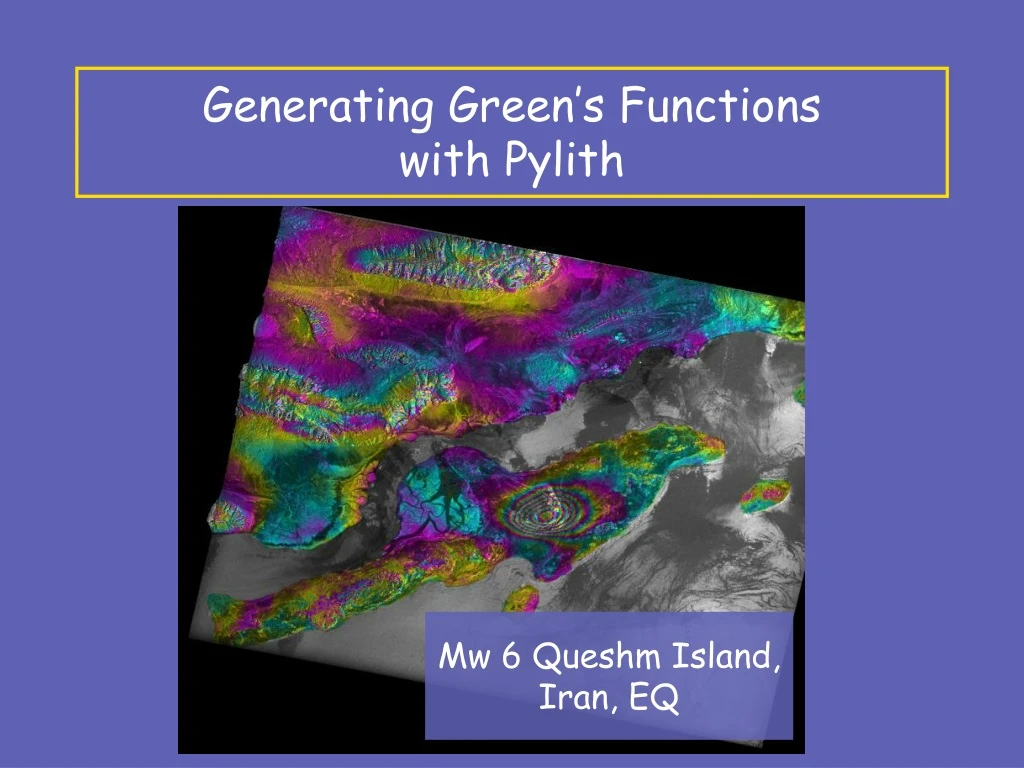
1. Generating Green’s Functions with Pylith Mw 6 Queshm Island, Iran, EQ

2. Outline • Overview/Motivation • When/where use FE models? • Workflow • From data to mesh to Green’s functions to model • Examples • Bam & Qeshm Island earthquakes, Iran Astronaut photography http://eol.jsc.nasa.gov/

3. Effects of Crustal Structure • Vertical layering (2D) • Tends to move apparent source up or down (~10% effect) • Horizontal contrasts (3D) • Map into slip features, inferred geometry • Fialko (2006) finds 2-2.5x contrasts in So. Cal • Goal: For generic settings, what is inversion sensitivity? • Generate synthetic data using cross-fault contrast • Find best-fit solution in elastic half space • Assess bias: Inferred fault dip

4. Choosing Model Complexity • Case 1 • Lots of info • Seismicity • Velocity/rigidity structure • Mapped faults • Atmospheric water vapor content • Computationally expensive…. Community fault model So. Cal

5. Choosing Model Complexity • Case 2: • Sparse information • Mainly teleseismic EQ locations • No continuous GPS • Sporadic remote sensing Bam EQ, courtesy E. Fielding

6. Case 1: How do we use all this information? When do we have to include all info? When does it make sense to simplify? Case 2 What bias do we introduce by using inadequate models? How should we present this error? Which problems can we still address? Choosing Model Complexity

7. FE Workflow • Step 1: Matlab • Define data/fault geometry • Define crustal structure • Subdivide fault • One patch at a time, build Cubit, Pylith input files Vertical, strike-slip fault, divided into patches

8. Okada-based Green’s functions Slip on shallow fault patch

9. Okada-based Green’s functions Slip on deep fault patch

10. Inversion

11. FE Workflow • Step 2: Cubit • Build mesh • Step 3: Pylith • Generate Green’s functions • Step 4: Matlab • Assemble all patches, perform inversion

12. FE Workflow • Step 2: Cubit • Build mesh • Step 3: Pylith • Generate Green’s functions • Step 4: Matlab • Assemble all patches, perform inversion

13. FE Workflow • Step 2: Cubit • Build mesh • Step 3: Pylith • Generate Green’s functions • Step 4: Matlab • Assemble all patches, perform inversion Mesh quality/density?

14. Comparison w/Okada • Discrete fault patches • Readily available (Okada, Poly3D) • Easy to visualize • Historical:compare with previous work • Node, points • More natural comparison once Pylith Green’s functions mode

15. Comparison w/Okada 3D version • Discrete fault patches • Readily available (Okada, Poly3D) • Easy to visualize • Historical:compare with previous work • Node, points • More natural comparison once Pylith Green’s functions mode

16. Comparison w/Okada • More misfit from shallower ramp • Can fit almost exactly with different fault patch

17. Comparison w/Okada • More misfit from shallower ramp • Can fit almost exactly with different fault patch

18. Comparison w/Okada • More misfit from shallower ramp • Can fit almost exactly with different fault patch

19. Comparison w/Okada • More triangular -> wider patch w/ less slip • Moments/centroid almost identical

20. Examples: Sensitivity Tests • Generate synthetic data using cross-fault contrast (slow) • Invert using half space (fast) • Assess potential bias

21. Examples: Sensitivity Tests • Generate synthetic data using cross-fault contrast (slow) • Invert using half space (fast) • Assess potential bias

22. Examples: Sensitivity Tests • Generate synthetic data using cross-fault contrast (slow) • Invert using half space (fast) • Assess potential bias

23. Vertical Fault Deformation Patterns Can’t fit asymmetric pattern with vertical fault Apparent dip: 75º

24. Cross-Fault Contrast Results • Retrieve input geometry when contrast=0 • Up to 20 degree error for reasonable values • Sensitivity depends on noise RMS, viewing geometry

25. Cross-Fault Contrast Results • Retrieve input geometry when contrast=0 • Up to 20 degree error for reasonable values • Sensitivity depends on noise RMS, viewing geometry

26. 11/27/05, Mw 6 Qeshm Island EQ Zagros Mtns Qeshm Persian Gulf Astronaut photography http://eol.jsc.nasa.gov/

27. 11/27/05, Mw 6 Queshm Island EQ Color scale = 2.8 cm

28. 11/27/05, Mw 6 Queshm Island EQ Color scale = 40 cm

29. Assessing Potential Bias in Inferred Dip Error from noise Error from structure Atmospheric noise > Structure error

30. 2003 Bam, Iran, Earthquake • > 40 cm line-of-sight deformation • Not much structural/fault location info • How well do inversions for fault dip perform? Data courtesy Eric Fielding

31. 2003 Bam, Iran, Earthquake • Pylith: • Generate Green’s functions for distributed slip inversion • Repeat for various dip angles, cross-fault contrasts

32. 2003 Bam, Iran, Earthquake • Increased contrast = increased dip • Best fit still no-contrast solution, near-vertical dip • Geometrical irregularities = large residual • Need more complicated geometry before can assess crustal contribution

33. Conclusions • Sensitivity tests can largely be done with analytic inversions • More time consuming FE modeling (especially inversions) can be avoided for many problems • Large atmospheric noise • Known fault plane geometry • Patch by patch Green’s function generation very time consuming • Can be a bit more efficient, use redundant dip/strike info • Internal Pylith Green’s function producer very desirable