Download
1 / 26
260 likes | 274 Vues
This article revisits and applies a previous analysis to SECCHI-like observations, using coronal models and imaging-rendering techniques to investigate the solar stereographic mission.

E N D
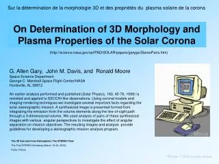
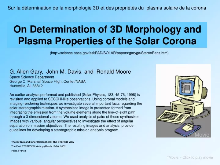
Sur la détermination de la morphologie 3D et des propriétés du plasma solaire de la corona On Determination of 3D Morphology and Plasma Properties of the Solar Corona (http://science.nasa.gov/ssl/PAD/SOLAR/papers/garyga/StereoParis.htm) G. Allen Gary, John M. Davis, and Ronald Moore Space Science Department George C. Marshall Space Flight Center/NASA Huntsville, AL 36812 An earlier analysis performed and published (Solar Physics, 183, 45-76, 1998) is revisited and applied to SECCHI-like observations. Using coronal models and imaging-rendering techniques we investigate several important facts regarding the solar stereographic mission. A synthesized image is presented formed from integrating the emission from the volume elements along the line-of-sight path through a 3-dimensional volume. We used analysis of pairs of these synthesized images with various angular perspectives to investigate the effect of angular separation on mission objectives. The resulting images and analysis provide guidelines for developing a stereographic mission analysis program. Movie The 3D Sun and Inner Heliosphere: The STEREO View The First STEREO Workshop (March 18-20, 2002) Paris, France *Movie – Click to play movie
Conclusions 3D(x,y,t) 4D(x,y,z,t) nD(x,y,z,t,,T,v,B,..) Temporal set of stereographic 2D images to a MHD physical model – the challenge (EUVI analysis as per paper but CORs analysis is complex ) A priori information – The all important input Location of centroid (large-scale structures) Principal axis of symmetry (origin: near or far-side) Principal axis of radial expansion (evolutionary track) Region of origin and footpoints Temporal history Global magnetic field Specific triangularization (location) of point sources (micro-structures) Physical nature of the object Observational constraints Self-similar modeling Serendipity – The magic of the mission
STEREO- Solar Terrestrial Relations Observatory +1yr Launch of Dual Spacecrafts: 5 May 2006 Launch Solar-B: 5 OCT 2005 Mission Concept: The STEREO mission will provide a totally new perspective on solar eruptions and their consequences for Earth. Achieving this perspective will require moving away from our customary Earth-bound lookout point. To provide the images for a stereo reconstruction of solar eruptions, one spacecraft will lead Earth in its orbit and one will be lagging. Each will carry a cluster of telescopes. When simultaneous telescopic images are combined with data from observatories on the ground or in low Earth orbit, the buildup of magnetic energy, and the lift off, and the trajectory of Earthward-bound CMEs can all be tracked in three dimensions. When a CME reaches Earth's orbit, magnetometers and plasma sensors on the STEREO spacecraft will sample the material and allow investigators to link the plasmas and magnetic fields unambiguously to their origins on the Sun. Mission Scientist Davila-GSFC SECCHI (Sun Earth Connection Coronal and Heliospheric Investigation) is a suite of remote sensing instruments consisting of two white light coronagraphs (1.2-3 and 3-15 Rs) and an EUV imager (2x EIT), collectively referred to as the Sun Centered Imaging Package, and a heliospheric imager (12-84Rs; 66-318Rs). PI Howard-NRL SWAVES (Stereo Waves) measures interplanetary type II and type III radio bursts, both remotely and in situ. Type II radio bursts are associated with the propagation of CMEs in the corona and interplanetary medium (IPM). PI Bougert-CNRS,France IMPACT (In-situ Measurements of Particles and CME Transients) includes a Solar Wind (SW) experiment to measure ~0-100 keV electrons, a magnetometer (MAG) experiment to measure the vector magnetic field, and a Solar Energetic Particle (SEP) experiment to measure electrons and ions. PI Luhmann-UCB PLASTIC (PLasma And SupraThermal Ion Composition investigation) measures solar wind protons and alphas, the elemental composition, charge state distribution, kinetic temperature, and velocity of heavy ions, and measures suprathermal ions. PI Galvin-UNH
Review of Previous Analysis Gary, Davis, & Moore,1998, Solar Phys. 183, 45 Synthesized coronal loop images of optical thin flux tubes • Conclusions of that analysis: • Maximum information at a specific angular separation • Benefits of time - differential imaging • A priori information improves volume reconstruction 0o 10o 30o 45o 60o 90o Stereographic Pairs Employing time separated images
Review of Previous Analysis Gary, Davis, & Moore,1998, Solar Phys. 183, 45 Tomography by Discrete Reconstruction Techniques (See paper for details) Frey’s Modified Multiplicative Algebraic Reconstruction (MART) Importance of temporal subtractive techniques and a priori information Restricted volume based on magnetic field extrapolation Three-view of the render coronal loops seen along the x, y, and z axes. (Top triplet: Input model Bottom triplet: Derived model)
Data Analysis Flow of coronal loops: Triangulation Magnetic Field Extrapolation Coronal Rendering Tomographic analysis Iteration • 3D geometric location • Interacting loops located. • 3D direction of motion determined. • Importance of photospheric motion. • Nonpotentiality magnetic field determined. • Foot points of coronal loops determined. • Determine the 3D dynamical changes in the coronal structure. • Determined the importance of flux emergence and reconnection of CMEs. • Assesses the important of dynamical change and configuration on coronal heating. • Density and temperature models.
Scientific Objectives Achieved at Each Step High Cadence Time Series Stereo Images Analysis of geometric structures in 3D of coronal loops, coronal walls, helmet streamers, and coronal mass ejections Interacting loops located or discounted. 3D direction of motion determined. Foot points determined by downward extrapolation. Importance of photospheric features on heating of coronal loops established. Nonpotentiality of the magnetic field determined by comparison with potential, force-free, and MHD models. Foot points determined by downward extrapolation of the correct magnetic model Determine the 3D dynamical changes in the coronal structure. Determined the importance of flux emergence and reconnection of CMEs. Assesses the important of dynamical change and configuration on coronal heating. Models for density and temperature of the coronal loops. Triangulation (x,y,z) Magnetograms (Bl,B) Build magnetic field models (potential, force-free, MHD) Set of coronal loops and features in 3D Disagrees Check consistency of magnetic boundary conditions Linear comparison of observed and calculated loops and features Modify magnetic boundary conditions to correct magnetic model Agrees 3D magnetic field model Physical scaling laws consistent with multi-temperature images Physics based rendering of loops and features to form synthesized images Render surface of loops and features Reiterate Resolving cores loops via disassembling loops and using solar rotation Image comparison of rendered and observed images Comparison criteria passed Full 3D coronal model based on least-square image analysis Tomographic analysis via Multiplicative Algebraic Reconstruction Techniques (MART) High cadence time series Full 3D coronal model which is fully compatible with stereographic images Physical characteristics of coronal loops Full 3D dynamical model of the corona [x,y,z,t,T,r]
SXT image type Gary (1997) Solar Physic 174, 241 Various Instrumental Response Functions Movie EIT image Type
Large Scale vs. Fine Scale Structure Solar & Heliospheric Observatory Large Angle Spectrographic Coronagraph “Light Bulb” 1.5Rs 1.0Rs C2 1999-10-12 11:50UT C2 2000-02-7 09:42UT C2 1998-12-08 14:30UT C2 1998-06-02 13:31UT
Deformation models & standardizing against similarity transformations Coronal Transient Models Mouschovias & Poland (1978,AJ,200,657) Coronal loop Pneuman (1980,SP,65,369) Coronal loop Gibson & Low (1998,AJ,493,460) Closed bubble +… Wu et al. (2000,AJ,545,1101) Closed bubble+… CME Ejection Models Subclass I Subclass II Storage and Release Models: 1) Mass loading and release 2) Magnetic tether release 3) Magnetic tether straining Directly Driven Models: 1) Thermal impulsive blast 2) Dynamo inflation Ref: Klimchuk, J. A., 2001, Geophys. Mono. 125, AGU
Movies Simple Synthesized Models ►Optically thin ► Fixed, random fine structure ► Added point sources (Large scale vs small scale) Closed Bubble Movies Simple Synthesized Models Movie Coronal Loop with core Closed Bubble with core Point source Movie Movie
A priori information: Location of centroid (large-scale structures) Principal axis of symmetry (origin: near or far-side) Principal axis of radial expansion (evolutionary track) Region of origin and footpoints Temporal history Velocity Vector Global magnetic field Specific triangularization (location) of point sources (micro-structures) Physical nature of the object Classification: CME, streamers, plumes Temporal evolution: Expansion rates Density constraint (positive definite, maximum density limit) Continuity – connectivity - cohesiveness of features. Observational constraints Limit on micro-structures (spatial resolution) Density gradients Self-similar models A priori information:
The discrete reconstruction problem: Estimate x given y y = R x + e Image pixels data Volume vector Noise Geometry projection matrix y00 Kth pixel y300 MinC2(x) = | y-R x |2 +g|x|2 +… Regularization Iterative Solution: x(l+1)= Pl( x(l) , R, y) vixons y = y00 y300 mth voxel y00k = rk1 x1+ rk2 x2+… +rnk xn Slice x: xm= xij(N2 voxels) Simple Epipolar Geometry
The discrete reconstruction problem y = R x + e Penalized Residual Minimization Problem MinC2(x) = | y-R x |2 + g |x C(p) x| .... C(p)= D(p) TD(p) where D(p) is the difference matrix to generate the Pth derivative. The inverse problem for STEREO: Minimization of the solution space. How to describe the “Penalized Residual Minimization Problem” taking into account the a priori information? And What is the best iterative method to employ to solve for a solution?
Iterative methods x2 ART Algebraic Reconstruction Technique pseudo-projection y001 = r11 x1+ r12 x2 X0 Initial guess X0 2-voxel example MART y1 y2 Multiplicative Algebraic Reconstruction Technique y3002 = r21 x1+ r22 x2 x1 x2 x1 MART: xi(l+1)= xi(l) [yi / (rk,x(l))]g cycle k, k=row (projection) , l =iteration, 0<g<1 ART: x(l+1)= x(l) + [yk-(rk,x(l))] rk/ (rk,rk) cycle k, k=row (projection), l =iteration =relaxation parameter
Backward Projection Radon transform: y(, )= -x[ cos +s sin , sin +s cos )] d s Backward projection: xB(, )= 0y[, cos + sin )] d The output xB is the volume x blurred by the Radon transform. Reference IDL routine: RADON ds Movie m=2 m=3 m=4 m=5 m=6 m=9
MART: Multiplicative Algebraic Reconstruction Technique ►Initial Guess of all the emission values via backward projection ► Updating scheme by modifying elements ► Elements which have zero emission remain void ► Result yields reconstruction with lowest information content for the voxels consistent with the given images, i.e., the solution of the maximum-entropy problem. The desire is to use all the a priori information and the 3D input of a series of time images of an event and reconstruct an 4D representation (e.g., the volume as a function of time) of the coronal transient.
Stereographic Pairs 300 Separation A priori information = Volume A priori information= none X Y Z X Y Z Model Model Back projection Back projection Frey’s MART Frey’s MART
Stereographic Pairs 300 Separation A priori information = Shape A priori information= Volume (~9%) X Y Z X Y Z Model Model Back projection Back projection Frey’s MART Frey’s MART
Stereographic Pairs 900 Separation A priori information = Shape X Y Z Model Back projection Frey’s MART
Time-differential imaging Reference: Dere, K. P., et al. 1999, ApJ, 516,465,Fig. 5 Cause of variations Line of Sight effects Density fluctuations Multiple events Background Movie
“Image” of CME at Fixed Radius A Time Coronal Mass Ejection 11-Nov-96 Ref. Simnett, G. M, et al. 1997, Solar Phys.,175, 685, CD Rs=5.5 B Movie Are there similarity transformations associated with CME outflow which can defined the associated volume? Rs=5.5 A Rs=3.0 Same Pre-Post Streamer ? B Rs=3.0
TRACE movie of filament eruption Movie Plasmaplot Movie Plasma beta model over an active region. The plasma beta as a function of height is shown shaded for open and closed field lines originating between a sunspot of 3000 G and a plage region of 150 G. What role does this-transition play in the CME early evolution? (Ref. Gary, G. A., 2002, Solar Phys., 203, 71)
The PTA Concept: Parametric Transformation Analysis (PTA) A Concept of Magnetic Field Solution PTA parametrically transforms a magnetic field solution to another solution which matches the coronal features by preserving on the divergence condition of the field. Movie Improving the field line alignment with the coronal loops with a radial stretching (transformation) of the field lines. Ref. Gary, G. A., & Alexander, D., 1999,Solar Physics, 186, 123.
Conclusion: 3D(x,y,t) 4D(x,y,z,t) nD(x,y,z,t,,T,v,B,..) Temporal set of stereographic 2D images to a MHD physical model – the challenge A priori information – The all important input Location of centroid (large-scale structures) Principal axis of symmetry (origin: near or far-side) Principal axis of radial expansion (evolutionary track) Region of origin and footpoints Temporal history Global magnetic field Specific triangularization (location) of point sources (micro-structures) Physical nature of the object Observational constraints Self-similar modeling Serendipity – The magic of the mission
Merci pour votre attention. Thank you for your attention.