The Full Steiner Tree Problem

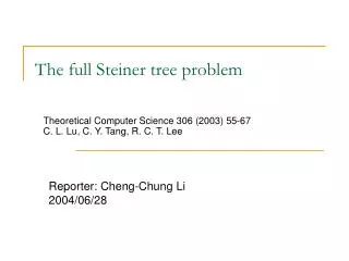
1. The Full Steiner Tree Problem Chin-Lung Lu, Chuan-Yi Tang, Richard, Chia-Tung Lee Theoretical Computer Science, Vol. 306, 2003, pp.55-67. Speaker: Chuang-Chieh Lin Advisor: Professor Maw-Shang Chang Dept. of CSIE, National Chung-Cheng University October 1, 2004

2. Outline • Introduction • Preliminaries • Hardness results • An -approximation algorithm • Conclusion • References

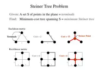
3. Introduction • Given a graph G = (V, E), a subset R  V of vertices, and a length function d: E+ on the edges, a Steiner tree is a connected and acyclic subgraph of G which spans all vertices of R. • The vertices in R are usually referred to as terminals and the vertices in V \ R as Steiner (or optional) vertices. • Note that a Steiner tree might contain the Steiner vertices.

4. The length of a Steiner tree is defined to be the sum of the lengths of all its edges. • The so-called Steiner tree problem is to find a Steiner minimum tree. (i.e., a Steiner tree of minimum length) in the given graph G. • For example,

5. 5 6 5 2 2 2 3 4 3 2 2 4 13 : terminals : Steiner vertices The length of this Steiner tree is 2+2+2+2+4=12.

6. Another Steiner tree 5 6 5 2 2 2 3 4 3 2 2 4 13 : terminals : Steiner vertices The length of this Steiner tree is 4+2+2+3+4=15.

7. Applications:([CD2001], [DSR2000], [FG82], [HRW92]) • VLSI design • Network routing • Wireless communications • Computational biology • This problem has been proved to be NP-complete, even in the Euclidean metric or rectilinear metric.[K72]

8. Motivated by the reconstruction of phylogenetic (or evolutionary) tree in biology, we study a variant of the Steiner tree problem, called the full Steiner tree problem (FSTP). • A Steiner tree is full if all terminals are leaves of the tree. • FSTP is to find a full Steiner tree with minimum length. • For example,

9. 5 6 5 2 2 2 3 4 3 2 2 4 13 The Steiner tree shown above is right a full Steiner tree with minimum length 12.

10. 5 6 5 2 2 2 3 4 3 2 2 4 13 The Steiner tree shown above is also a full Steiner tree with minimum length 12.

11. From the viewpoints of biologists, the terminals of a full Steiner tree T can be regarded as the extant taxa (or species, morphological features, biomolecular sequences), the internal vertices of Tas the extinct ancestral taxa, and the length of each edge in Tas the evolutionary time along it. • According to the principle of parsimony, T corresponds to an evolutionary tree of the extant species, which trends to minimize the tree length. • The principle of parsimony: Nature always finds the paths that require a minimum evolution.

12. If we restrict the lengths of edges to be either 1 or 2, then the problem is called the (1, 2)-full Steiner tree problem (FSTP(1, 2)). • Little work has been done on the FSTP.

13. In this paper, FSTP(1, 2) will be shown to be NP-complete and MAX SNP-hard. Therefore FSTP is surely NP-complete and MAX SNP-hard. • However, an -approximation algorithm for the FSTP(1, 2) is shown in this paper. (Its running time is polynomial but it is NOT a PTAS)

14. Preliminaries • To make sure that a full Steiner tree exists, we restrict the given graph G = (V, E) to be complete and R to be a proper subset of V (i.e., RV ) • We assume that the length function d is a metric.

15. The length function d is called a metric if it satisfies the following three conditions: • d(x, y)  0 for any x, y in V, where equality holds iff x = y • d(x, y) = d(y, x) for any x, y in V • d(x, y)  d(x, z) + d(z, y) for any x, y, z in V (triangular inequality)

16. Let us see the problems again.

17. FSTP: • Given a complete graph G = (V, E), a length function d: E+ on the edges, a proper subset RV, and a positive integer bound B. Is there a full Steiner tree T in G such that the length of Tis less than or equal to B? • MIN-FSTP: • Given a complete graph G = (V, E), a length function d: E+ on the edges and a proper subset RV of terminals, find a full Steiner tree of minimum length in G. • MIN-FSTP(1, 2): • Given a complete graph G = (V, E), a length function d: E{1, 2} on the edges and a proper subset RV of terminals, find a full Steiner tree of minimum length in G.

18. In order to proceed to the proof the hardness results, we have to be familiar with the following concepts: • L-reduction • Performance ratio • Polynomial time approximation scheme (PTAS) • MAX SNP-hard

19. L-reduction • Given two optimization problems Π1 and Π2, we say that Π1L-reduces to Π2if there are polynomial-time algorithms f and g and positive constants αandβ such that for any instance I of Π1, the following conditions are satisfied: • Algorithm f produces an instance f(I) of Π2 such that OPT(f(I))  αOPT(I), where OPT(I) and OPT(f(I)) stand for the optimal solutions of I and f(I), respectively. • Given any solution of f(I) with cost (size) c2, algorithm g produces a solution of I with cost (size) c1 in polynomial time such that |c1OPT(I)|β|c2OPT(f(I))|.

20. I : an instance of Π1 f(I) : an instance of Π2 sI: a solution of I sf(I) : a solution of f(I) g f sf (I) I f(I) sI size c1 size c2 OPT(f(I))  αOPT(I) |c1OPT(I)| β|c2OPT(f(I))|.

21. Performance ratio • Given an optimization problem P, for any instance x of P and for any feasible solution y of x, the performance ratio of y with respect to x is defined as where m*(x) denotes the measure of an optimal solution of instance x and m(x, y) denote the measure of solution y.

22. PTAS • Let P be an optimization problem. An algorithm A is said to be a polynomial-time approximation scheme (PTAS) for P if, for any instance x of P and any rational value r >1, A, when applied to input (x, r), returns an r-approximate solution of x in time polynomial in |x|. (r is the performance ratio) • A problem has a PTAS if for any fixed r > 1, the problem can be approximated within a factor of r in polynomial time (polynomial in |x|; r is the performance ratio).

23. MAX SNP-hard • Here we omit the precise definition. • A problem is said to be MAX SNP-hard if a MAX SNP-hard problem can be L-reduced to it. • Note: • If P  NP, then there doesn’t exist any PTAS for any MAX-SNP-hard problem. • If there were a PTAS for one of the MAX SNP-hard problems, there were a PTAS for all of them.

24. Hardness results • We will show that the optimization problem MIN-FSTP(1, 2) is MAX SNP-hard by an L-reduction from the vertex cover-B problem (VC-B for short), which was shown to be MAX SNP-hard by Papadimitriou and Yannakais in 1991. [PY91] • VC-B: Given a graph G = (V, E) with degree bounded by a constant B, find a vertex cover of minimum cardinality in G.

25. Let G1=(V1, E1) and B be an instance I1 of VC-B with V1 = {v1, v2, …, vn} (WLOG, we assume that G1 is connected and n3.) Then we transform I1 into an instance I2 of MIN-FSTP(1, 2), say G2 and R, as follows. • A complete graph G2 = (V2, E2) with V2 = V1{zi,j | (vi,vj)E1}, and R = V2\V1 = {zi,j | (vi,vj)E1}. • For each edge eE2, d(e) = where  = {(vi,vj) | 1i<jn}{(vi.,zi,j), (zi,j,vj) | (vi,vj)E1}. (This is right the polynomial-time transformation algorithm f which will be mentioned later.)

26. Let us see an example.

27. : terminal v1 v1 z1,2 z1,5 v2 v2 v5 v5 z4,5 z2,3 v4 v3 v4 v3 z3,4 G1 G2 An L-reductionfrom VC-B to MIN-FSTP(1, 2). Note that only edges of length 1 in G2 are shown for simplicity.

28. Lemma 1 • Let T be a solution of length c to MIN-FSTP(1, 2) on the instance I2 which is obtained from a reduction of an instance I1 of VC-B. Then in polynomial time, we can find another solution T 'of length no more than c to MIN-FSTP(1, 2) on instance I2 such that T 'contains no edge of length 2.

29. Proof • In the following proof, we only show how to replace an edge of length 2 from T with some edges of length 1 in polynomial time without increasing the length of the resulting T . • By repeatedly applying this procedure to T , we will finally obtain T 'in polynomial time.

30. y v1 z1,2 z1,5 v2 v5 z4,5 z2,3 x v4 v3 z3,4 Let (x, y) be an edge of length 2 in T . One of x and y must be a terminal and the other must be a Steiner vertex. WLOG, we assume that x is a terminal and y is a Steiner vertex.

31. Since G1 is connected and n3, x must be connected to some one terminal z with a path of two edges of length 1, say (x, v) and (v, z). Let u be the Steiner vertex of which is adjacent to z. Then we consider the following two possibilities. Case 1: u=v d(x, v)=1 d(x, y)=2 v1 = y v1 = y z1,2 z1,2 z1,5 z1,5 v2 v2 v5 v5 z4,5= x z4,5= x z2,3 z2,3 v4 = u = v v4 = u = v v3 v3 z3,4 = z z3,4 = z

32. Case 2: uv d(x, y)=2 d(x, v)+ d (v, u) = 1+1=2 v1 = y v1 = y z1,2 z1,2 z1,5 z1,5 v2 v2 v5 v5 z4,5 = x z4,5 = x z2,3 z2,3 v4 = v v4 = v v3 = u v3 = u z3,4 = z z3,4 = z

33. Theorem 1 • MIN-FSTP(1, 2) is a MAX SNP-hard problem. • Proof: • Let f denote the polynomial-time algorithm to transform an instance I1 of VC-B to the instance I2 of MIN-FSTP(1, 2). • We design another polynomial-time algorithm g as follows.

34. Given a full Steiner tree in TinG2 of length c,we transform it into another full Steiner tree T 'using the method described in the proof of Lemma 1. • Collect the internal vertices of T 'which are adjacent to the leaves of T '.

35. Clearly, T 'contains no edge of length 2 and its length is no more than c. • Then we know that the number of vertices in T 'is less than or equal to c+1 since T 'is a tree. • The collection of those internal vertices of T ',which are adjacent to the leaves of T ',corresponds to a vertex cover of G1 whose size is less than or equal to c|E1|+1.

36. v1 z1,2 z1,5 v2 v5 z4,5 z2,3 v4 v3 z3,4 A Steiner tree is shown by red edges of the graph above. The corresponding vertex cover of G1 is {v2, v3, v5}.

37. Next, we will show that algorithms f and g are an L-reduction from VC-B to MIN-FSTP(1, 2). • (1) OPT(f(I1))  αOPT(I1), where α= 2B: • B OPT(I1)  |E1| since each vertex in G1 covers at most B edges. • Let u be a vertex in G1 whose degree is B. Then let us build a “star”Ψwith u as its center and R as its leaves. Clearly, Ψ is a feasible solution of MIN-FSTP(1, 2) on f(I1).

38. v1 z1,2 z1,5 • The length of Ψis B + 2(|E1|  B) = 2|E1|  B. • Hence, v2 v5 B = 2 z4,5 z2,3 v4 v3 z3,4 Since B OPT(I1)  |E1|

39. (2) |c1OPT(I1)| β|c2OPT(f(I1))|, where β= 1: • Given a vertex cover VC in G1 of size c, we can create a full Steiner tree in G2 of length c+|E1|1 in the following way. • Step 1: Connect each edge of E1 (corresponding to a terminal in G2) to an arbitrary vertex in VC (corresponding to a Steiner vertex in G2) • Step 2: Connect all vertices of VC by c1 edges of length 1 in G2.

40. v1 z1,2 z1,5 : vertex cover VC v2 v5 c = 3 • Hence, OPT(f(I1))  OPT(I1)+|E1|1 since the right part of this inequality formula is the length of a Steiner tree of f(I1), while OPT(f(I1)) stands for the length of the “optimal ” Steiner tree of f(I1). • Don’t forget that OPT(I1) +|E1|1 c+|E1|1 z2,3 z4,5 Step 2 v4 v3 Step 1 z3,4

41. By algorithm g, a full Steiner tree of G2 with length c2 can be transformed into a vertex cover of G1 of size c1, where c1 c2|E1|+1. • Then, we obtain that • Hence,

42. Now, we have shown that MIN-FTSP(1, 2) is MAX SNP-hard. • MIN-FSTP is certainly MAX SNP-hard.

43. An -approximation algorithm • Any star with an arbitrary Steiner vertex as its center and all terminals as its leaves is an approximate solution with performance ratio within 2 of the optimal one. (We can consider that |E1|  OPT(f(I1))  2B OPT(I1) and |E1|  B OPT(I1)) • Instead, we will give an -approximation algorithm for MIN-FSTP(1, 2) using the so-called average length heuristics. [BP89, RS83]

44. Steiner star: • A star T with Steiner vertex as its center and the terminals as its leaves • Xk-star: • A Steiner star T with k leaves and d(center(T ), v) = 1 for each v of leaves(T ) • Average length f(T ): • For a Steiner tree T with |leaves(T )|2, 1 1 1

45. The above definition can be regarded as a kind of scoring function for Steiner stars. • After giving the above definitions, let us proceed to some important lemmas.

46. Lemma 2: Let T be a Steiner star with k terminals, where k2. If T contains no leaf at distance 1 from center(T ), then f(T ) = 2+2(k1). • Lemma 3: Let T be a Steiner star with k terminals, where k2. If T contains only one leaf at distance 1 from center(T ), then f(T ) = 2+1(k1). • Lemma 4: Let T be a Steiner star with k terminals, where k2. If T contains exactly two leaves at distance 1 from the center(T ), then f(T )=2. • Lemma 5: Let T be a Xk-star with k3. Then f(T )= 1+1(k1). • Lemma 6: Let T1 be a Xk-star with k3 and let T2be the Steiner star obtained from T1 by adding a new terminal z with d(center(T1), z)=2. Then f(T1)<f(T2).

47. Since it is not hard for us to prove the lemmas, we omit the proofs here. • Now, let us go to see the algorithm directly.

48. Algorithm APX-FSTP(1,2) • Input: A complete graph G=(V, E) with d: E{1,2} and a set RV of terminals • Output: A full Steiner tree TAPX for R in G. • Step 1: Let  be an empty set; • Step 2: /* Choose a Steiner star with the minimum average length */ if there are two or more remaining Steiner vertices then find a Steiner star Twith the minimum average length; iff(T)=2 then /*Transform T into an X2-star*/ Remove from T those leaves at distance 2 from center(T) end if else Let T be the Steiner star with the only Steiner vertex as its center and remaining terminals as its leaves;

49. Step 3:/*Perform a reduction*/ Let  =  {(center(T ), v) | vleaves(T )} Replace the Steiner star T by a single new terminal, say z; Let d(z, u)=d(center(T ),v) for each remaining vertex u; • Step 4: if there is still more than one terminal then Go to Step 2; • else Let TAPX be the full Steiner tree induced by ; • end if

50. For example, consider the following figure. 2 1 2 2 1 1 1 1 1 2