Download
1 / 64
640 likes | 807 Vues
A Simple Model of Subtropical Stratocumulus Cloud Feedbacks. Peter Caldwell and Chris Bretherton NCAR CGD Seminar 10/23/08. UCRL: LLNL-PRES-407609. Motivation:. Annual-Average Low Cloud Amount. Net Cloud Radiative Forcing *. Low clouds cover large regions of the globe.

E N D
A Simple Model of Subtropical Stratocumulus Cloud Feedbacks Peter Caldwell and Chris Bretherton NCAR CGD Seminar 10/23/08 UCRL: LLNL-PRES-407609
Motivation: Annual-Average Low Cloud Amount Net Cloud Radiative Forcing* Low clouds cover large regions of the globe (graphics courtesy Steve Klein) and have the strongest cloud radiative forcing. * Cloud radiative forcing = clear-sky flux – observed flux (both at top of atmosphere)
Low Clouds Worst Simulated: • 500mb ω is an indicator of Sc Subsidence Rate ω @ 500mb (mb day-1) From CCSM3.0 A1B (Oct 2000-2010) Spread in Tropical-Ocean Cloud-Forcing Trends from 15 Ocean-Atmosphere GCMs Stratocumulus Deep Convection 30ºN ΔCloud Forcing (W m-2 K-1) 30ºS high sensitivity models low sensitivity models -50 -25 0 25 50 Subsidence Rate ω @ 500mb (mb day-1) from Bony & Dufresne (GRL 2005) • Spread in cloud forcing is largest in Sc regime
drizzle damps turbulence, dries out BL Why this Uncertainty? Entrainment (BL growth due to incorporation of free-tropospheric air by turbulent eddies) dries, warms BL Gravity waves homogenize θ across tropics Free Troposphere 10K! Cloud-top LW cooling induces turbulence ~2000 km separation Deep convection sets θ to ~moist adiabat Boundary Layer (BL) BL θ close to local SST Stratocumulus (Sc) Region Intertropical Convergence Zone (ITCZ)
drizzle damps turbulence, dries out BL Why this Uncertainty? 1.Interaction between turbulence, radiation, and microphysics hard to parameterize Entrainment (BL growth due to incorporation of free-tropospheric air by turbulent eddies) dries out cloud Gravity waves homogenize θ across tropics 3.Sc changes depend on largest and smallest scales Free Troposphere 12K! Cloudtop LW cooling induces turbulence Deep convection sets θ to ~moist adiabat 2.Important scales not resolved in GCMs Boundary Layer (BL) BL θ close to local SST Stratocumulus (Sc) Region Intertropical Convergence Zone (ITCZ)
Simple Models • Why a Simple Model Might Work: • Free-tropospheric T easy to parameterize from ITCZ SST • Constant relative humidity assumption (Held and Soden, 2000) allows specification of qv • Subsidence can be obtained from free-tropospheric energy budget • Previous studies have exploited these features(e.g. Betts and Ridgway, JAS 1989, Pierrehumbert, JAS 1995, Miller, JC 1997, Larson et al., JC 1999): • 2xCO2 response: • -Hadley circulation slows • Warm-cold ΔSST ↑ • LTS↑ Sc cloud ↑ from Larson et al. (1999)
Our Model • Shared with previous studies: free-tropospheric • - temperature • - moisture • - subsidence • Differs by: • Using a more realistic BL model • Accounting for radiative effect of cold BL on air just above cloud top. • NOT including Sc→ITCZ feedback (gives extra free parameter) from Larson et al. (1999)
Outline: • Motivation • Model Introduction • Validation Data • Explanation/Validation of Model Components • Temp • Moisture • Subsidence • Mixed Layer Model (MLM) • Results • Uniform SST increase • Slab-ocean case • Comparison against GCMs • Conclusions
Data – Observations @ 20°S, 85°W: • EPIC = East Pacific Investigation of Climate (Oct. 2001) http://www.atmos.washington.edu/~caldwep/research/ScDataset/sc_integ_data_fr.htm 2. PACS ’03 = Pan-American Climate Studies (Nov. 2003) Similar, but 6 hourly radiosondes, no scanning radar, and better aerosol measurements. 3. PACS ’04 = Pan-American Climate Studies (Dec. 2004) Similar, but ~11 days of 6 hourly radiosonde data. 6 days of 3 hrly radiosondes, vertical and scanning radar, microwave radiometer, shipboard measurements obtained aboard the NOAA vessel Ronald H. Brown.
Obs Param Tropical Temperature Structure: EPIC Region (20°S, 85°W) • Observationally, tropical temperature follows a modified moist adiabat(Betts QJRMS, 1982) • modification due to lateral entrainment, detrainment in convecting plumes EPIC PACS ‘03 PACS ‘04 Moist Adiab Modified Moist Adiab
Lapse Rate Feedback • Warmer air holds more moisture • greater condensational warmer in rising parcels • temperature perturbations increase with height • This feedback is well studied (e.g. Hansen et al., GM 1984).
Free-Tropospheric Moisture EPIC Region (20°S, 85°W) Param • 10% RH fits the EPIC data reasonably well • Moistureis highly variable in time Obs
Free-Tropospheric Subsidence Outside of the BL, radiation is the only energetic forcing on a parcel, so In steady state = 0, leaving where = horiz. advection, = subsidence rate = net radiative heating rate
Subsidence Parameterization Radiative heating calculated from free-tropospheric profiles using BUGSrad, a 2-stream correlated-k scheme where = horiz. advection, = subsidence rate = net radiative heating rate
Subsidence Parameterization Potential Temp is modified moist adiabatic Radiative heating calculated from free-tropospheric profiles using BUGSrad, a 2-stream correlated-k scheme where = horiz. advection, = subsidence rate = net radiative heating rate
Subsidence Parameterization Horiz. advection idealized from Sept-Nov average ERA40 data at 20S, 85W. Assumed independent of climate change. Potential Temp is modified moist adiabatic Radiative heating calculated from free-tropospheric profiles using BUGSrad, a 2-stream correlated-k scheme where = horiz. advection, = subsidence rate = net radiative heating rate
Subsidence Parameterization Horiz. advection idealized from Sept-Nov average ERA40 data at 20S, 85W. Assumed independent of climate change. Residual is subsidence rate! Potential Temp is modified moist adiabatic Radiative heating calculated from free-tropospheric profiles using BUGSrad, a 2-stream correlated-k scheme where = horiz. advection, = subsidence rate = net radiative heating rate
Detail #1 The previous method neglects BL effects, so it doesn’t satisfy ws(0)=0. To correct for this, we force ws to decrease linearly from its calculated value at z*= 1.8km (z* = smallest z>zi in all runs) to 0 at the surface:
Corrected Uncorrected ERA40 Detail #2: Proximity to the cold BL significantly enhances radiative flux divergence just above zi. This: • decreases θ • increases ws This effect is parameterized by computing the ws and θ perturbations induced by the radiative enhancement assuminglinear hydrostatic f-plane dynamics and sinusoidal latitudinal variation in diabatic heating. EPIC Obs Uncorrected Corrected All enhancement → cooling
constant increases ~constant Current SST+2K Subsidence Feedback Subsidence should decrease as the planet warms Recent papers supporting this conclusion: Knutson and Manabe (JC, 1995), Zhang and Soon (GRL, 2006), Held and Soden (JC, 2006), Vecchi et al. (N, 2006)
BL Model details • Cloud-topped mixed layer model (MLM, Lilly,QJRMS 1968) – fully consistent model of BL dynamics if: • -Liquid water potential temperature and total water mixing ratio are constant in height • -Horizontally homogenous (cloud fraction 0 or 1) • Bulk surface fluxes with ||v||=6.2m s-1 (tuned to get ocean heat flux right) • BL advection fixed with: • Fully interactive 2-stream correlated-k radiation (BUGSrad) • Comstock et al. (QJRMS, 2004) drizzle parameterization with Rogers and Yau (1989) Stokes’ flow droplet sedimentation • Turton-Nicholls entrainment closure with Bretherton et al. (GRL, 2007) sedimentation correction • MLM run to steady state. Wyant et al. (JAMES 2008) suggests constant as climate changes
How to Read Results: Balanced Surface Budget Contours of constant zi Current Climate Equal Warming
negative buoyancy flux Measured by the buoyancy integral ratio (BIR) = positive buoyancy flux 305 304 303 302 301 300 299 0<BIR<0.15: well mixed according to Bretherton + Wyant (JAS 1997) BIR=0: well mixed according to Stevens (GRL 2000) SST in ITCZ region BIR>0.15: not well mixed 289 290 291 292 293 294 295 SST in stratus region Domain of Validity: Buoyancy Flux (w’b’): are turbulent motions enhanced or damped by buoyancy? Condensation, LW cooling result in large w’b’ in cloud evaporation, entrainment can make w’b’ <0 below cloud base
Results: • Black line (Cess): equal SSTstrat and SSTITCZ warming. • BL deepens and LWP increases →Negative feedback on global warming
Why does LWP increase along 1:1 line?: Reason 1:For large we, we increases zi more than zb • Entrainment decreases difference between BL and free troposphere, decreasing the impact of further entrainment fluxes • Entrainment also damps BL turbulence, which should increase BL stratification (but MLM doesn’t do this)
Why does LWP increase along 1:1 line?: Reason 2: Warming increases adiabatic liquid water for fixed zi, zb (Somerville and Remer, JGR 1984) • dql/dz can be computed using Clausius-Clapeyron, well-mixedness • Accounts for <10% LWP rise in our simulations
Why does LWP increase along 1:1 line?: Reason 3: Decrease in subsidence at warmer SSTITCZ allows cloud to thicken (subsidence/lapse-rate feedback) • newly discovered feedback described on next slide
ws pushes the BL down we forces the BL up Ocean Subsidence/Lapse-Rate Feedback 1. Subsidence weakens as SSTITCZ rises. This causes zi to grow. 2. Inversion strength (θ+ - θBL) increases with rising zi. 4. Decreased entrainment drying, warming lowers zb. inversion strengthens 5. Rising zi, sinking zb increases LWP. θe higher zi lower zi LWP high LWP low Ocean 3. Increased inversion stability results in we decrease. Ocean
Results: • Red line (slab ocean): model forced to obey surface energy balance, ocean transport fixed at current conditions (37 W m-2 into ocean). Assume constant • Decrease in surface insolation with rising LWP now allowed to feed back, causing • local SST to rise more slowly than ITCZ SST • BL depth to decrease • weaker LWP rise than in Cess case.
CMIP3 A1B SST Response GCM Model Name: All models start here Stratus region = Average over 10-20º S, 80-90º W ITCZ region = Precipitation-weighted Pacific Ocean average • Suggests no Sc feedback in GCMs • Is definition of Sc region representative? • Are other processes driving SST change? • Does cloud shading increase with rising SST?
CMIP3 A1B SST Response CMIP3 Composite 21st Century SST Change from A1B Scenario 24 12 0 -12 -24 0 30 60 90 120 150 180 210 240 270 300 330 360 ΔSST (K): 0.9 1.2 1.5 1.8 2.1 2.4 • Warming is moderate in core SE Pacific Sc region (pink box) • Top 10% LTS regions (white contours) show varied SST response, with average similar to top 10% precip regions (black contours) Sc feedback not governing GCM SST change
CMIP3 Composite 21st Century SST Change from A1B Scenario 24 12 0 -12 -24 0 30 60 90 120 150 180 210 240 270 300 330 360 ΔSST (K): 0.9 1.2 1.5 1.8 2.1 2.4 CMIP3 Composite 21st Century SW CRF Change from A1B Scenario 24 12 0 -12 -24 0 30 60 90 120 150 180 210 240 270 300 330 360 ΔSW CRF (W m-2): -9 -6 -3 0 3 6 More Shading Less Shading Does Cloud Shading Control GCM SST? • Cloud shading not dominant factor in SST change • Less SW CRF (so less low clouds) in Sc regions
SE Pacific Sc Region ΔSW CRF 15 4.2 12 3.9 9 3.6 3.3 6 3 Equilibrium Clim. Sensitivity (K) SW CRF Trend (W m-2 century-1) 3 2.7 0 2.4 -3 2.1 ipsl_cm4 ncar_pcm1 inmcm3_0 gfdl_cm2_0 miub_echo_g ukmo_hadgem1 mpi_echam5 gfdl_cm2_1 csiro_mk3_0 iap_fgoals1_0_g miroc3_2_hires ncar_ccsm3_0 cccma_cgcm3_1 ukmo_hadcm3 giss_model_e_h miroc3_2_medres mri_cgcm2_3_2a cccma_cgcm3_1_t63 Change in SW CRF by Model Only 4 of 18 models show increased cloud shading in SE Pacific Sc core as SST rises! Why? • MLM could be wrong: • Cloud fraction fixed at 0 or 1 • increase in stratification with BL depth not included • GCMs could be wrong: • GCM low clouds result from a complex mixture of parameterizations (e.g. Zhang and Bretherton JC,2008) This is important because models with positive Δ SW CRF in SE Pacific tend to have higher climate sensitivity
Future Work • Use more sophisticated BL model to include stratification, cloud fraction • current GCSS/CFMIP intercomparison project • Check how well my parameterizations are followed by GCMs • trends in advection, surface winds, etc which should be included in simple model? • basic processes not captured in GCMs?
Conclusions • Presence of BL requires important modifications to simple 2-box model • With MLM, our system generally predicts increased LWP and hence negative feedback on global warming • GCMs tend to show positive feedback on warming • Failure to capture intermediate cloud fractions and observed increase in stratification with rising zi may be playing a role
Conclusions (cont’d) • Uniform SST increase → large rise in LWP due to: • zb insensitivity at higher we • increased LWP with warming at fixed zi, zb • subsidence lapse-rate feedback • Slab ocean assumption → • weak local SST increase (due to cloud shading) • decreased zi (due to increased inversion strength) • damped LWP rise (due to lower zi) • Sc response depends on pattern of SST change!
Thanks! Details in Caldwell and Bretherton (accepted, J. Climate 2008) A copy of our paper and this .ppt is available at www.atmos.washington.edu/~caldwep/Research.html
But Low Clouds Increase in CAM, right? Climate Change in CAM2.02_rio33 (SST+2 – Control) Δcloud fraction (%) Δcloud water content (g kg-1) • CAM low cloud increase is primarily outside of the core Sc regions Results from Wyant et al. (CD, 2007) Δ CRF (W m-2)
Comparison against AR4 sresa1b GCM Model Name: • CCSM does show weaker SST rise in SE Pacific • Wyant et al. (CD, 2006) found similar results for GFDL AM2.12b, GMAO NSIPP-2 • Seen here to be outside core Sc region (as defined by Klein and Hartmann (JC, 1993) • Suggests cloud shading is not reason for cooling October SST Trend (K century-1) From 1st century of CCSM3.0 A1B SST Trend (K century-1) Stratus region = Average over 10-20º S, 80-90º W -3 -2.4 -1.8 -1.2 -0.6 0 0.6 1.2 1.8 2.4
Tropical Low Cloud response to ENSO • El Nino decreases clouds where SST increases • Because stability is increased • Graphic includes all ocean between 40S and 40N (MLM not appropriate) • Since ENSO SST pattern not like that for climate change, ENSO of limited use for diagnosing climate change • El Nino decreases Walker circulation, but increases E. Pac Hadley circulation (Wang, 2004) • Unclear what happens to circulation From Zhu et al. (JGR, 2007)
Free Tropospheric Correction *=horiz perturbation geopot. • Linearize f-plane equations about a free-tropospheric reference state (geostrophic, radiative cooling balances subsidence warming) • assume perturbation cooling only varies in x direction so d/dy=0 rad cooling perturbation 0=reference (BL-free) state
Free Tropospheric Correction *=horiz perturbation geopot. 2. Take D/Dl of eq 1, sub into eq 2 to eliminate v*. Take d/dx of result and substitute eq 4 to get rid of u*. Result: rad cooling perturbation 0=reference (BL-free) state
Free Tropospheric Correction *=horiz perturbation geopot. 3. Use steady-state and scaling argument to get rid of Dl2/Dt2 in the equation below. 4. Substitute eq 3 on right to get function of θ*and ω*. rad cooling perturbation 0=reference (BL-free) state
Free Tropospheric Correction This yields: 5. Scale analysis shows last 2 terms in summand can be ignored 6. Assume Q*, θ*and ω* have spatial distribution where X=Q, θ, or ω, primes are perturbations at the model location, and Λis the width of the cooling perturbation (~distance btwn ITCZ and Sc region). Substitute into above eq and evaluate at x=0.
Free Tropospheric Correction Combine with thermodynamic equation to get: where is the forcing and is a Rossby adjustment pressure depth for given Λ. We use P0= 300mb to get realistic subsidence at 1km. This corresponds to f at 15°lat, Λ=1650 km, and S0=0.04K/mb at 500mb.
Effect of Entrainment Param. Nicholls-Turton Nicholls-Turton Nicholls-Turton Lewellen Lewellen Lewellen -Entrainment parameterization has little effect on dynamics.
Effect of Drizzle • Tested by varying droplet concentration (Nd) since Less droplets → average drop larger→ falls faster→ more precip 1st indirect aerosol effect Results: • Small ctrl-run drizzle rates → weak response to Nd changes • Cloud response to Nd depends on LWP Drizzle DECREASES LWP LWP|Nd=100/cc – LWP|Nd=50/cc LWP|Nd=100/cc Drizzle INCREASES LWP (Ackerman et al. 2004)
Effect of Drizzle Fractional change in optical depth due to changing Nd = + 1st indirect aerosol effect Effect of spreading given LWP over more droplets (1st indirect aerosol effect) Effect due to changing LWP (2nd indirect aerosol effect) LWP|Nd=100/cc – LWP|Nd=50/cc LWP|Nd=100/cc 2nd indirect aerosol effect much weaker than 1st