Download
1 / 20
200 likes | 447 Vues
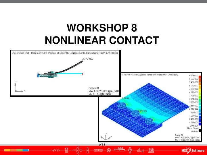
WORKSHOP 8 NONLINEAR CONTACT. Workshop Objectives Learn how to run a nonlinear (Solution 400) analysis Investigate the difference between glued and touching contact Software Version MSC SimXpert R3 Files Required contact_linear.SimXpert Problem Description

E N D
Workshop Objectives • Learn how to run a nonlinear (Solution 400) analysis • Investigate the difference between glued and touching contact • Software Version • MSC SimXpert R3 • Files Required • contact_linear.SimXpert • Problem Description • The contact analysis in Workshop 13 assumed that the plates were bonded together, leading to inaccurate results • In this workshop the model needs to be modified to allow the plates to separate • The analysis will be run using a nonlinear static solution
Suggested Exercise Steps • Enter SimXpert Structures Workspace. • Open existing Simxpert file contact_linear.SimXpert • Create a contact table. The bolts are glued to the plates. The plates can separate from each other. • Set up a general nonlinear analysis • Run the finite element analysis using MD Nastran. • Check the status of the job by reviewing the .f06 file • Attach the .xdb file • Plot displacements • Plot stresses. • Compare Linear and Nonlinear Results • Save the database as contact_nonlinear.SimXpert.
Step 1. Enter the SimXpert Structures Workspace Open the SimXpert Structures Workspace • Click on Structures a
Step 2. Open an Existing SimXpert File a Open the nonlinear contact SimXpert database • Select File > Open • Navigate to and select contact_linear.SimXpert. • Click Open. b c
Step 3. Create a Contact Table a Define Glue option between the bolts and plates and Touch option between the plates. • Under the LBC’s tab, select Table from the Contact group • For Name enter Glue_Bolts • Click Glue All. • Click Deact. Diagonal to eliminate self-contact. • Since the bolts will not come into contact with each other, in row 1 (bolt_1) clear columns 2 and 3 by repeatedly clicking in each box until it is blank. In row 2 (bolt_2) clear column 3 by clicking in the box until it is blank. • In row 5 (top plate) change column 4 to ‘T’ by clicking in the box until it is changed. • Click OK. b d c e f g
Step 4. Setup a Nonlinear Analysis b a Specify analysis parameters. • Right-click the FileSet and select Create new Nastran Job. • Enter contact_nonlinear as the Job Name. • Select General Nonlinear Analysis (SOL400) for the Solution Type. • Click the folder icon to to the right of the Solver Input File text box. • Select the file path to where the Nastran job will be saved. • Enter contact_nonlinear in the File name textbox. • Click Save. • Click OK c d h e f g
Step 4. Setup a Nonlinear Analysis (Cont.) Specify analysis parameters. (continued) • Collapse the contact_linear job tree • Under the contact_nonlinear job tree, right click on Loads/Boundaries and select Select BCTABLE • Select Glue_Bolts from the Model Browser • Click OK. c c a d b
Step 4. Setup a Nonlinear Analysis (Cont.) Specify analysis parameters. (continued) • Right-click on Solver Control and select Properties. • Select ContactControlParameters • Check Activate Quadratic Contact • Click Apply. • Click Close. a b c d e
Step 4. Setup a Nonlinear Analysis (Cont.) Specify analysis parameters. (continued) • Right-click Loadcase Control and select Properties. • Select Sol400SubcaseNonlinearStaticParameters • Set Number of Load Increments to 2. • Set Total Time to 1.0. • Click Apply. • Click Close. a b c d e f
Step 5. Run Analysis Run Analysis • Right click on contact_nonlinear and select Run. a
Step 6. Check the Progress • Open the f06 file using a text editor. If you cannot open the f06 because it is in use, create a copy of the file and open the copy. • Scroll to the end of the file. • If the job is still running you should see the iteration output table. • The LOAD STEP column indicates how much of the current load step it is attempting to solve. A value of 0.5 indicates that 50% of the load is being applied in this increment. • The number of iterations it has performed is shown in the ITR column. • When the job finishes, you will see a message confirming job convergence. d e f
Step 7. Attach the Results b e Attach the .xdb file to access the analysis results. • Select File > AttachResults. • Click the Folder icon for FilePath. • Navigate to and select the file contact_nonlinear.xdb • Click Open. • Select Results as the Attach Option. • Click OK. a f c d
Step 8. Results - Deformation Plot a Deformation Plot. • Under the Results tab, select Deformation. • In Result cases select the contact_nonlinear.xdb job • Select Results Type Displacements, Translational. • Click the DeformationTab • Select True for Deformed display scaling. • Click Update to show the true deformation. c b d e f
Step 8. Results - Deformation Plot (Cont.) a Deformation Fringe Plot (Cont.) • Orient the model to Left View and zoom in to check separation between plates. • Change the value of True to 10 to see the separation exaggerated. • Click Update • Click Clear when finished. c b d
Step 9. Results - Stress Fringe Plot a b f d e c Generate a Stress Fringe Plot • Click the Plot Data tab • Select Fringe as the Plot type. • Select contact_nonlinear.xdb as the Result Case • Change Result type to Stress Tensor. • Select von Mises for Derivation: • Click Update. • Orient the model to Isometric view. g g f
Step 10. Compare Linear and Nonlinear Results a h b f g e i Compare the nonlinear results with the linear results. • Select Window >New Window • Select Window > Tile • Click the frame of the Structures window to make it current • Select contact_linear.MASTER as the Result Case • Select Result type Stress Tensor. • Select von Mises for Derivation: • Click Update. • Click Clear and close the State plot property editor. • When you have finished viewing the results, click Clear • Close the Structures Window c j
Step 10. Compare Linear and Nonlinear Results (Cont.) Compare the nonlinear results with the linear results. (Cont.) • Right-click Plot Fringe 01 in the Model Browser and select Delete • Answer Yes to the Delete Fringe 01? prompt. a b
Step 11. Save the Database a Save the database to continuelater in the Nonlinear Material Workshop • Select File > SaveAs • Enter File Name contact_nonlinear • Click Save. • Select File > Exit d b c