Download
1 / 54
540 likes | 677 Vues
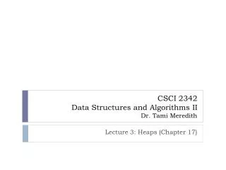
CSCI 2342 Data Structures and Algorithms II Dr. Tami Meredith. Lecture 1: Trees (Chapter 15). Terminology. Trees represent relationships Trees are hierarchical in nature “Parent-child” relationship exists between nodes in tree Generalized to ancestor and descendant

E N D
CSCI 2342Data Structures and Algorithms IIDr. Tami Meredith Lecture 1: Trees (Chapter 15)
Terminology • Trees represent relationships • Trees are hierarchical in nature • “Parent-child” relationship exists between nodes in tree • Generalized to ancestor and descendant • Lines between the nodes are called edges • nodes = entities • edges = relationships • A subtree in a tree is any node in the tree together with all of its descendants • A node with no children is often referred to as a leaf
FIGURE 15-1 (a) A tree (b) a subtree of the tree in part A Terminology
FIGURE 15-2 (a) An organization chart (b) a family tree Terminology
Kinds of Trees • General Tree • Set T of one or more nodes such that T is partitioned into disjoint subsets • A single node r, the root • Sets that are general trees, called subtrees of r
Kinds of Trees • n-ary tree • set T of nodes that is either empty or partitioned into disjoint subsets: • A single node r, the root • n possibly empty sets that are n-arysubtrees of r • n is the degree of the tree, i.e., the maximum number of children a node can have
Kinds of Trees • Binary tree • Set T of nodes that is either empty or partitioned into disjoint subsets • Single node r, the root • Two possibly empty sets that are binary trees, called left and right subtrees of r • An n-ary tree of degree 2
FIGURE 15-3 Binary trees that represent algebraic expressions Example: Algebraic Expressions.
Binary Search Tree • For each node n, a binary search tree (BST) satisfies the following three properties: • n’s value is greater than all values in its left subtree TL • n’s value is less than all values in its right subtree TR • Both TL and TR are binary search trees
FIGURE 15-4 A binary search tree of names Example: Binary Search Tree
The Height of a Tree • Definition of the level of a node n: • If n is the root of T, it is at level 1 • If n is not the root of T, its level is 1 greater than the level of its parent • Height of a tree T: • If T is empty, its height is 0 • If T is not empty, its height is equal to the maximum level of any node • i.e., the number of nodes on a direct path to the farthest leaf
FIGURE 15-5 Binary trees with the same nodes but different heights The Height of Trees
Full Binary Tree • Definition of a full binary tree • If T is empty, T is a full binary tree of height 0 • If T is not empty and has height h > 0, T is a full binary tree if its root’s subtrees are both full binary trees of height h–1 • A tree is full when all nodes, except the leaves, have two children and all leaves are at the same level • FIGURE 15-6 A full binary tree of height 3
FIGURE 15-7 A complete binary tree Example: Complete Binary Tree
Complete Binary Tree • A tree of height h such that • All nodes at level h-2 and above have 2 children • If a node at level h-1 has children, all nodes to its left at the same level have two children and if it has only one child, it is a left child • A tree that it is full to height h-1 and level h is filled from left to right
The maximum height of an n-node binary tree is n FIGURE 15-8 Binary trees of height 3 The Maximum Height of a Binary Tree
FIGURE 15-9 Counting the nodes in a full binary tree of height h The Maximum and Minimum Heights of a Binary Tree
Facts about Full Binary Trees • A full binary tree of height h ≥ 0 has 2h – 1 nodes • You cannot add nodes to a full binary tree without increasing its height • The maximum number of nodes that a binary tree of height h can have is 2h – 1 • The minimum height of a binary tree with n nodes is [log 2 (n + 1)]
Traversals of a Binary Tree • General form of recursive traversal algorithm • This algorithm provides preorder traversal and can be modified to perform 2 different variations • All 3 traversals are forms of depth-first search
Traversals of a Binary Tree • Preorder traversal
Traversals of a Binary Tree • Inorder traversal
Traversals of a Binary Tree • Postorder traversal
FIGURE 15-11 Traversals of a binary tree Example: Traversals of a Binary Tree
Main Binary Tree Operations • Test whether a tree is empty • Get the height of the tree • Get the number of nodes in the tree • Get the data in a tree's root • Set the data in a tree's root • Add a new node containing a given data item to a tree • Remove the node containing a given data item from a tree • Remove all nodes from the tree (i.e., delete the tree) • Retrieve a specific entry in a tree (i.e., search the tree) • Test whether a tree contains a specific entry (i.e., search the tree) • Traverse the nodes in preorder, inorder, or postorder
FIGURE 15-12 UML diagram for the class BinaryTree Binary Tree Operations
The ADT Binary Search Tree • General binary trees are inefficient when searching for specific item • Binary Search Trees (BSTs) solve the problem • Recall, for each node, n, of a BST • n’s value greater than all values in left subtreeTL • n’s value less than all values in right subtreeTR • Both TR and TL are binary search trees
FIGURE 15-13 A binary search tree of names Example: Binary Search Tree
Example: Non-Uniqueness of a BST FIGURE 15-14 Binary search trees with the same data as in Figure 15-13
Binary Search Tree Operations • Test whether BST is empty • Get height of a BST • Get number of nodes in a BST • Get data in BST's root • Insert new item into a BST • Remove given item from a BST • Remove all entries from a BST • Retrieve given item from a BST (i.e., search) • Test whether BST contains specific entry (i.e., search) • Traverse items in binary search tree in preorder, inorder, or postorder
template<class ItemType> class BinaryTreeInterface { public: virtual boolisEmpty() const = 0; virtual intgetHeight() const = 0; virtual intgetNumberOfNodes() const = 0; virtual ItemTypegetRootData() const = 0; virtual void setRootData(const ItemType& newData) = 0; virtual bool add(const ItemType& newData) = 0; virtual bool remove(const ItemType& data) = 0; virtual void clear() = 0; virtual ItemTypegetEntry(const ItemType& anEntry) const throw(NotFoundException) = 0; virtual bool contains(const ItemType& anEntry) const = 0 virtual void preorderTraverse(void visit(ItemType&)) const = 0; virtual void inorderTraverse(void visit(ItemType&)) const = 0; virtual void postorderTraverse(void visit(ItemType&)) const = 0; }; // end BinaryTreeInterface
Searching a Binary Search Tree • Search algorithm for binary search tree
FIGURE 15-15 An array of names in sorted order Creating & Searching a BST FIGURE 15-16 Empty subtree where the search algorithm terminates when looking for Frank
Creating a BST • Very simple two step process • Search for the item you wish to insert • Create a new node for the data and place the node as the appropriate child of the leaf where the search failed • If search finds the item, then it is in the tree and doesn't need to be added
Traversals of a Binary Search Tree • Algorithm
FIGURE 15-17 The Big O for the retrieval, insertion, removal, and traversal operations of the ADT binary search tree Efficiency of BST Operations
Notes on Efficiency • The more complete a tree is, the more efficient it is for searching • We always want to minimise the height of the tree as much as possible • Balanced trees of Chapter 19 address this issue (e.g., Red-Black Trees, AVL Trees) • Our existing insertion algorithm works best when data comes in a uniformly distributed random order
Summary • Root: The topmost node • Parent: The ancestor or node above • Child: The descendant or nodes below • Sibling: Nodes with the same parent • Leaf: A node with no children • Internal node: A node with at least one child • Degree: Number of subtrees/children of a node • Edge: Connection between two nodes • Path: A sequence of nodes and edges connecting any node with a descendant • Level: Number of edges from the root to a node (by the most direct path ) • Height: Length of the longest path in the tree • Forest: Two disjoint (unattached) trees
C and C++ • C++ originally cross-compiled to C • C++ is a superset of C (i.e., all C programs can be compiled by GPP) • C is really just a structured version of assembly language • C has very minimal library support compared to C++ • C was originally created as a language to program Unix (i.e., systems programming) • C was created by Brian Kernighan and Dennis Ritchie and C++ by BjarneStroustrup at Bell Labs • Developed before mice, GUI's; Designed for CLIs
The File Model • All C I/O is done using files • 3 special files are provided: stdin (cin), stdout (cout), and stderr (cerr) • These files are automatically opened and closed for you by the compiler • I/0 can be done directly using fread() and fwrite() • More useful to do formatted I/O using fprintf() and fscanf()
Formatted Output fprintf(file, “format”, values); • Various version of fprintf() exist: printf(...) is the same as fprintf(stdout,...) sprintf(): print to a string (or character buffer) v_printf(): variable number or args • Other output functions are also available: fputc(), putc(), putchar(), puts() Each function has its own subtleties
Formatted Output printf(“format”, args ...); • Format contains format specifiers, such as %d (integer), %s (string), %c (character) • There must be an argument for every specifier • Format can contain output modifiers such as \n to insert a newline printf(“%d is %s than %d\n”, i[0], “smaller”, max);
Conversions • s string • d signed integer • f float (double) • c single character • p pointer • Many others exist for alternative numeric formats • n displays the number of characters printed so far
ALL the Conversions ... • %c The character format specifier.%d The integer format specifier.%i The integer format specifier (same as %d).%f The floating-point format specifier.%e The scientific notation format specifier.%E The scientific notation format specifier.%g Uses %f or %e, whichever result is shorter.%G Uses %f or %E, whichever result is shorter.%o The unsigned octal format specifier.%s The string format specifier.%u The unsigned integer format specifier.%x The unsigned hexadecimal format specifier.%X The unsigned hexadecimal format specifier.%p Displays the corresponding argument as a pointer.%n Records the number of characters written so far.%% Outputs a percent sign.
Format Specifiers • % • flags (0ptional): sign, zero padding, etc. • minimum width (optional) • .precision (optional): maximum chars • length modifier (optional): short, long • argument type conversion: string, pointer, character, float, integer, etc. %-2.8hs, %d, %*s
Examples of Output printf ("Hello World\n"); char buf[256]; sprintf(buf,"%8d\t%8d", a, b); fprintf(stderr, "%s: fatal: %s not found", argv[0], argv[1]); FILE *log = fopen("log.txt","w+"); fprintf(log,"%s: %s\n", time, msg);
File Mode Values • "r" read • "w" write • "a" append • "r+" reading and writing • "w+" create then reading and writing and discard previous contents • "a+" open or create and do writing at end
C Input • To match fprintf() for output there is fscanf(file,fmt,args)for input. E.g., fscanf(stdin, “%s %d”, name, &grade); • Format specifiers are pretty similar, but do have a few differences • ArgsMUST be addresses (pointers) name is a char* grade is an int so we use its address
More on Input • Various versions of fscanf() exist • fscanf(stdin,...) same as scanf(...) • scanf()is hard to use at first! • Also have: fgetc(), getc(), getchar(), fgets(), gets(),andungetc() Each function has its own little quirks