Download
1 / 72
1.67k likes | 2.94k Vues
EEE3440-04 Digital Communications: Fall Semester 2012. Note 5. Channel Coding: Part 2 : Convolutional Codes. Sooyong Choi csyong@yonsei.ac.kr School of Electrical and Electronic Engineering Yonsei University. Channel Coding : Part 2. Simple Communication System.

E N D
EEE3440-04 Digital Communications: Fall Semester 2012 Note 5. Channel Coding: Part 2 : Convolutional Codes Sooyong Choi csyong@yonsei.ac.kr School of Electrical and Electronic Engineering Yonsei University
Simple Communication System • Encode/decode and modulate/demodulate portions of a communication link Information source Convolutional encode Modulate AWGN channel Information sink Convolutional decode Demodulate
Convolutional Codes • A Convolutional code is specified by three parameters or where • is the coding rate, determining the number of data bits per coded bit. • In practice, usually k=1 is chosen and we assume that from now on. • K is the constraint length of the encoder a where the encoder has K-1 memory elements. • There is different definitions in literatures for constraint length.
Convolutional Encoder • Rate = k/n = ½, K = 3 Convolutional Encoder Output branch Word U Input bit m
Convolutional Encoder • Generator polynomial • = Connection vector • = Encoding function • g1 = 1 1 1 • g1(X) = 1+X+X2 • Rate = k/n = ½, K = 3 + u1 : First code symbol Output branch Word U Input bit m u2 : Second code symbol • Generator polynomial • = Connection vector • = Encoding function • g2 = 1 0 1 • g2(X) = 1+X2 + Convolutional encoder
Convolutional Encoder • Example : At time 1 + u1 = 1 1 0 0 0 m = 1 u2 = +
Convolutional Encoder • Example : At time 2 + 0 u1 = 1 0 1 0 m = 1 u2 = +
Convolutional Encoder • Example : At time 3 + 0 u1 = 0 1 1 0 m = 1 u2 = +
Convolutional Encoder • Example : At time 4 + 0 u1 = 1 1 0 1 m = 0 u2 = +
Convolutional Encoder • Example : At time 5 + 0 u1 = 1 0 1 1 m = 1 u2 = +
Convolutional Encoder • Example : At time 6 + 0 u1 = 0 1 1 0 m = 1 u2 = +
Convolutional Encoder • Example : At time 7 + 1 u1 = 0 1 0 1 m = 1 u2 = +
Effective Code Rate • Block code : A fixed word length n • Convolutional code : No particular block size • Initialize the memory before encoding the first bit (all-zero) • Clear out the memory after encoding the last bit (all-zero) • Hence, a tail of zero-bits is appended to data bits : No information • Effective code rate : • L is the number of data bits and k=1 is assumed: Encoder data tail codeword
Encoder Representation • Vector representation: • We define n binary vector with K elements (one vector for each modulo-2 adder) • The ith element in each vector, is “1” if the ith stage in the shift register is connected to the corresponding modulo-2 adder, and “0” otherwise. • Example:
Input m Output Modulo-2 sum: Encoder Representation • Impulse response representation: • The response of encoder to a single “one” bit that goes through it. • Example: Branch word Register contents Output = Superposition or the input addition of the time shifted input “impulses” Convolutional codes are linear
Encoder Representation • Polynomial representation: • Define n generator polynomials, one for each modulo-2 adder. • Each polynomial is of degree K-1 or less. • Each polynomial describes the connection of the shift registers to the corresponding modulo-2 adder. • Example: • Lowest order term in the polynomial = Input stage of the register • Output sequence :
State Diagram • Convolutional encoder A class of devices known as finite-state machines • Finite-state machines have a memory of past signals • A finite-state machine only encounters a finite number of states • State of a machine • The smallest amount of information that, together with a current input to the machine, can predict the output of the machine • The state provides some knowledge of the past signaling events and the restricted set of possible output in the future • Convolutional encoder :the state represented by the content of the memory • states • A state diagram is a way to represent the encoder • A state diagram contains all the states & all possible transitions between them • Only two transitions initiating from a state • Only two transitions ending up in a state
State Diagram + u1 m u2 0/00 + Output (Branch word) Input 00 1/11 0/11 1/00 10 01 0/10 1/01 0/01 11 Input bit 0 Input bit 1 1/10
Tree Diagram • State Diagram • Cannot represent time history • Tree Diagram • State diagram + dimension of time • Traversing the diagram from left to the right at each successive input bit time. • Input : Zero Its branch word : Moving to the next rightmost branch in the upward direction • Input : One Its branch word : Moving to the next rightmost branch in the downward direction Input = 11011
Trellis Diagram • Trellis diagram • Extension of the state diagram that shows the passage of time • Label each node : Four possible states in the shift register a = 00, b = 10, c = 01, and d = 11 • Tree structure : Repeats after K (= constraint length) branching • Sold line : Output generated by an input bit zero • Dashed line : Output generated by an input bit one • All branches emanating from two nodes of the same state generate identical branch word sequences Input bit 0 Input bit 1
Trellis Diagram • Nodes of the trellis • Characterize the encoder states • First row nodes : State a = 00 • Second & subsequent rows : States b = 10, c = 01, and d = 11. • Each unit of time : 2K-1 nodes to represent the 2K-1 possible encoder states • After depth K : Fixed structure • Branches of the trellis • Code symbol sequence • Characterized by N branches (representing N data bits) : N intervals of time Input bit 0 Input bit 1
Trellis Diagram • Encoder trellis diagram with rate k/n = ½, K = 3 State t1 t2 a = 00 b = 10 c = 01 d = 11 + u1 = 0 0 0 0 0 m = 0 u2 = +
Trellis Diagram • Encoder trellis diagram with rate k/n = ½, K = 3 State t1 t2 00 a = 00 b = 10 c = 01 d = 11 + u1 = 0 0 0 0 m = 0 u2 = +
Trellis Diagram • Encoder trellis diagram with rate k/n = ½, K = 3 State t1 t2 00 a = 00 b = 10 c = 01 d = 11 + u1 = 1 1 0 0 0 m = 1 u2 = +
Trellis Diagram • Encoder trellis diagram with rate k/n = ½, K = 3 State t1 t2 00 a = 00 b = 10 c = 01 d = 11 + 11 u1 = 1 0 1 0 m = 1 u2 = +
Trellis Diagram • Encoder trellis diagram with rate k/n = ½, K = 3 State t1 t2 t3 00 00 a = 00 b = 10 c = 01 d = 11 + 11 11 u1 = 1 0 0 1 X m = 0 u2 = +
Trellis Diagram • Encoder trellis diagram with rate k/n = ½, K = 3 State t1 t2 t3 00 00 a = 00 b = 10 c = 01 d = 11 + 11 11 u1 = 1 1 0 0 m = 0 u2 = 10 +
Trellis Diagram • Encoder trellis diagram with rate k/n = ½, K = 3 State t1 t2 t3 00 00 a = 00 b = 10 c = 01 d = 11 + 11 11 u1 = 0 1 0 1 X m = 1 u2 = 10 +
Trellis Diagram • Encoder trellis diagram with rate k/n = ½, K = 3 State t1 t2 t3 00 00 a = 00 b = 10 c = 01 d = 11 + 11 11 u1 = 0 1 1 0 m = 1 u2 = 10 + 01
+ Trellis Diagram u1 m u2 • Encoder trellis diagram with rate k/n = ½, K = 3 + State t1 t2 t3 t4 t5 t6 00 00 00 00 00 a = 00 b = 10 c = 01 d = 11 11 11 11 11 11 11 11 11 00 00 00 10 10 10 10 01 01 01 01 01 01 01 10 10 10
Convolutional Decoding • We talked about: • Another class of linear codes, known as Convolutional codes. • We studied the structure of the encoder and different ways for representing it. • State Diagram • Tree diagram • Trellis Diagram • From now on, we are going to talk about: • How the decoding is performed for Convolutional codes? • What is a Maximum likelihood decoder? • What are the soft decisions and hard decisions? • How does the Viterbi algorithm work?
Block Diagram of the DCS Information source Rate 1/n Conv. encoder Modulator Channel Information sink Rate 1/n Conv. decoder Demodulator
Formulation of the Convolutional Decoding Problem • Maximum Likelihood Decoding • All input message sequences are equally likely, • Decoder : Minimum probability of error • Compares the conditional probabilities called likelihood functions • : Received sequence • : One of possible transmitted sequences • Chooses the maximum • Maximum likelihood concept • Binary demodulation: Only two equally likely possible signals
Maximum Likelihood Decoding • Convolutional code • Has memory • Received sequence = Superposition of currents and prior bits • Applying ML = Choosing the most likely sequence • Multitude of possible codeword transmitted • Binary code • Sequence of L branch words = Member of a set of 2L possible sequences • ML decoder minimizes the error probability • Maximum likelihood • The decoder chooses a particular as the transmitted sequence if the likelihood is greater than the likelihoods of all other possible transmitted sequemces
Maximum Likelihood Decoding • Assumption • Additive white Gaussian noise with zero mean • Memoryless channel • Noise affects each code symbol independently of all the other symbols • Convolutional code of rate 1/n • Likelihood : • Zi : i th branch of the received sequence Z • : i th branch of a particular codeword sequence • zji : j th code symbol of Zi • : j th code symbol of • Each branch = n code symbols • The decoder problem : Choose a path through the trellis
Path metric Branch metric Bit metric Maximum Likelihood Decoding • Log-likelihood function • The decoder problem ⇒ Choose a path through the tree such that is maximized • Binary code • Sequence of L branch words = Member of a set of 2L possible sequences • Not practical to consider maximum likelihood decoding with a tree structure • The decoded path is chosen from some reduced set of surviving paths • Viterbi decoding algorithm • Performs maximum likelihood decoding • Optimal decoding
Channel Models: Soft & Hard Decisions • Hard decision • Demodulator • Makes a firm or hard decision whether one or zero is transmitted • Provides no other information for the decoder such that how reliable the decision is • Output of the demodulator : Only zero or one (the output is quantized only to two level) which are called “hard-bits” • Decoding based on hard-bits is called the “hard-decision decoding”.
Soft and Hard Decisions • Soft decision • Demodulator • Provides the decoder with some side information together with the decision • The side information provides the decoder with a measure of confidence for the decision • The demodulator outputs which are called soft-bits, are quantized to more than two levels • Decoding based on soft-bits, is called the “soft-decision decoding” • On AWGN channels, 2 dB and on fading channels 6 dB gain are obtained by using soft-decoding over hard-decoding
AWGN Channels • BPSK modulation • Transmitted sequence corresponding to the codeword is denoted by • Log-likelihood function • Maximizing the correlation = Minimizing the Euclidean distance Inner product or correlation between Z and S • ML decoding rule: Choose the path which with minimum Euclidean distance to the received sequence
The Viterbi Algorithm • Viterbi algorithm • Maximum likelihood decoding • Complexity : Not a function of the number of symbols in the codeword sequence • Calculating a measure of similarity or distance between the received signal at time ti and all the trellis paths entering each state at time ti • Find a path through trellis with the largest metric (maximum correlation or minimum distance). • Process the demodulator outputs in an iterative manner. • Compares the metric of all paths entering each state • Keeps only the path with the largest metric, called the survivor (surviving path), together with its metric. • Eliminate the least likely paths. • Goal of selecting the optimum path • Choosing the codeword with the maximum likelihood metric, or with the minimum distance metric
Viterbi Algorithm • Do the following set up: • Form the trellis for a data block of L bits • The trellis has L+K-1 sections or levels and starts at time t1 and ends up at time tL+K. • Label all the branches in the trellis with their corresponding branch metric • Define a parameter (S(ti), ti) for each state in the trellis at the time ti which is denoted by S(ti) {0, 1, 2,…, 2K-1} • Then, do the following: • Set (0, t1) = 0 and i = 2. • Compute the partial path metrics for all the paths entering each state at time ti • Set (S(ti), ti) equal to the best partial path metric entering each state at time ti Keep the survivor path and delete the dead paths from the trellis • If i < L+K, increase i by 1 and return to step 2. • Start at state zero at time tL+K • Follow the surviving branches backwards through the trellis. The path thus defined is unique and corresponds to the ML codeword
Example : Viterbi Decoding • Input data m: 1 1 0 1 1 • Codeword U: 11 01 01 00 01 Received seq. Z: 11 01 01 10 01 t1 t2 2 a = 00 b = 10 0
Example : Viterbi Decoding • Input data m: 1 1 0 1 1 • Codeword U: 11 01 01 00 01 Received seq. Z: 11 01 t1 t2 t3 1 2 a = 00 b = 10 0 1 2 0 c = 01 d = 11
Example : Viterbi Decoding • Input data m: 1 1 0 1 1 • Codeword U: 11 01 01 00 01 Received seq. Z: 11 01 01 t1 t2 t3 t4 1 1 2 a = 00 b = 10 0 1 1 1 1 2 2 0 c = 01 d = 11 0 0 2
Example : Viterbi Decoding • Input data m: 1 1 0 1 1 • Codeword U: 11 01 01 00 01 Received seq. Z: 11 01 01 t1 t2 t3 t4 1 1 2 Path metric a = 00 b = 10 0 1 1 4 1 1 2 3 2 0 c = 01 d = 11 0 0 2
Example : Viterbi Decoding • Input data m: 1 1 0 1 1 • Codeword U: 11 01 01 00 01 Received seq. Z: 11 01 01 t1 t2 t3 t4 1 1 2 Path metric a = 00 b = 10 0 1 1 4 1 1 2 3 2 0 c = 01 d = 11 0 0 2
Example : Viterbi Decoding • Input data m: 1 1 0 1 1 • Codeword U: 11 01 01 00 01 Received seq. Z: 11 01 01 t1 t2 t3 t4 1 1 2 a = 00 b = 10 0 1 1 Path metric 1 1 2 4 2 0 c = 01 d = 11 0 0 0 2
Example : Viterbi Decoding • Input data m: 1 1 0 1 1 • Codeword U: 11 01 01 00 01 Received seq. Z: 11 01 01 t1 t2 t3 t4 1 1 2 a = 00 b = 10 0 1 1 Path metric 1 1 2 2 0 c = 01 d = 11 0 3 2 0 2
Example : Viterbi Decoding • Input data m: 1 1 0 1 1 • Codeword U: 11 01 01 00 01 Received seq. Z: 11 01 01 01 t1 t2 t3 t4 t5 1 a = 00 b = 10 0 1 1 1 1 1 2 0 0 c = 01 d = 11 2 2 0 2 0