Download
1 / 96
990 likes | 1.46k Vues
Layer 3 The Network Layer. Slides adapted from Tanenbaum. Purpose of Internetworking. As we have seen, Layer 1 and Layer 2 networks are satisfactory for LAN level networks Bridges (layer2 switches) are used to match different Layer 2 protocols

E N D
Layer 3The Network Layer Slides adapted from Tanenbaum
Purpose of Internetworking • As we have seen, Layer 1 and Layer 2 networks are satisfactory for LAN level networks • Bridges (layer2 switches) are used to match different Layer 2 protocols • Bridges can also create Virtual LANs (VLANS) by grouping Hosts on different LAN segments through MAC level addressing.
Limitations of Layer2 switching • Even with complex bridges, NIC cards (hosts) never know the MAC address of all their possible destinations. • Frames get broadcast to everyone on the segment • Bridges filter somewhat, but may not know the exact host that should receive the Ethernet Frame (ends up wasting lots of bandwidth) • Layer 2 “Virtual LANs” (VLANs) only partially solve this. • Layer 2 networks don’t scale. • Complexity increases faster than number of nodes There’s got to be a better way.
Network Layer Design Issues • Store-and-Forward Packet Switching • Services Provided to the Transport Layer • Implementation of Connectionless Service • Implementation of Connection-Oriented Service • Comparison of Virtual-Circuit and Datagram Subnets
Store-and-Forward Packet Switching The environment of the network layer protocols. fig 5-1
Implementation of Connectionless Service Routing within a diagram subnet. Key point: Packet’s destination address is used to determine the required output port. Routing tables can change over time and packets can take different routes between the same two routers.
Implementation of Connection-Oriented Service Routing within a virtual-circuit subnet. Each switch looks at VCI and input port to determine the output port. Does not look at destination. This is like X.25, Frame and ATM VC switching that we saw before.
Routing Algorithms • The Optimality Principle • Shortest Path Routing • Flooding • Distance Vector Routing • Link State Routing • Hierarchical Routing • Broadcast Routing • Multicast Routing • Routing for Mobile Hosts • Routing in Ad Hoc Networks
Routing Algorithms (2) Conflict between fairness and optimality. If traffic flows between A and A’, B and B’, and C and C’, the utilization of the network will be good, but flow between X and X’ will be severely restricted. Fairness must often be imposed at the expense of overall utilization.
Optimality Principle • Optimality principle: • If router J is on the optimal path from router I to router K, then the optimal path from J to K also falls along the same route. • This means: • Given the final destination, routers only need to know the optimal route to the next router. • This entails a lookup-table correlating destination address and output port. • The following figure: • Shows the sink tree for destination “B” • There would be different sink trees for each final destination. • Note there are no loops in this tree.
The Optimality Principle (a) A subnet. (b) A sink tree for router B.
Shortest Path Routing The first 5 steps used in computing the shortest path from A to D. The arrows indicate the working node.
Shortest path routing • Algorithms that efficiently compute the shortest path • Dijkstra • Bellman • Another approach -- flooding may be used to send packets to all adjacent routers. • Packets that arrive at desired destination first are considered to have taken the “best”route. (this route is then chosen for subsequent packets.)
Distance Vector Routing • In a network of routers, the trick is to Adapt these algorithms to run in a distributed fashion. • Each router only needs to know who it’s connected to. • Doesn’t know the complete topology of the entire network. • Defining the “cost” of each link is an important consideration • Delay?? • Bandwidth?? • Real-cost?? • Queue-depth at input port of next router??
Distance Vector Routing • Each node builds up route tables with best output port and cost for all destinations of the network • In following slide J receives vectors from each neighbor • Also receives cost to those immediate neighbors • Looks at each possible route to every destination and selects lowest • Creates and stores the table locally • The “Count to Infinity” problem exists with distance vector routing • Each node is slow to realize a node has failed. • Split-horizon is a modification to alleviate this problem • Still doesn’t work perfectly RIP is an example of Distance Vector Routing Protocol
Distance Vector Routing (a) A subnet. (b) Input from A, I, H, K, and the new routing table for J.
Distance Vector Routing (2) The count-to-infinity problem, these vectors are the hops to A In (a), the router A has just come up, B learns then C, etc. (b) Shows what happens when A fails, each node is very slow to realize the cost to A is INFINITY.
Link State Routing Each router must do the following: • Discover its neighbors, learn their network address. • Measure the delay or cost to each of its neighbors. • Construct a packet telling all it has just learned. • Send this packet to all other routers. • Compute the shortest path to every other router.
Learning about the Neighbors (a) Nine routers and a LAN. (b) A graph model of (a).
Measuring Line Cost A subnet in which the East and West parts are connected by two lines. If link status is reported based congestion and distance, oscillations can occur. CF may be the best route so all traffic is moved over there. Then EI becomes a much better route, etc., etc., etc.
Building Link State Packets • With link-state routing, packets are created by each node that describe its adjacent links. • The AGE of the update and the sequence number are also included. • This allows changes in the network to be considered. • (a) A subnet. (b) The link state packets for this subnet.
Distributing the Link State Packets The packet buffer for router B in the previous slide Flooding is used to distribute link-state packets. As the link-state packets are flowing around the network, they must be managed. New ones are used to update and also sent on to adjacent nodes. Old ones are ignored and not forwarded. Using both Age and Sequence # prevents problems when routers reboot and lose sequence.
Hierarchical Routing Hierarchical routing. This type of architecture allows the routing protocols to scale. For example, all the flooded Link-state messages don’t have to propagate outside the areas.
Congestion Control Algorithms • General Principles of Congestion Control • Congestion Prevention Policies • Congestion Control in Virtual-Circuit Subnets • Congestion Control in Datagram Subnets • Load Shedding • Jitter Control
Basic Queuing Theory Arrivals • In a queue, things stack up as they are waiting to be serviced • Infinite length queues where the service rate is greater than the arrival rate produce a stable system. • The average waiting time for a M/M/1 queue is well known • In reality, things are different • Arrivals are not exponentially distributed • Data tends to be more bursty and “self-similar” (what is this?) • Real Queues can’t hold infinite number of messages (not enough memory, too much delay) • Multiple queues and priorities are implemented for QoS Servicing
Congestion • When queues in the Routers begin to be congested, measures must be taken to manage this. • Why not just let the queues overflow?? • Often this makes the problem worse • Flow control algorithms will try to resend further compounding the problem • Delay in the network would be maximum • Longer queues introduce more chance for Jitter • Lots of work has been done on congestion management
Congestion When too much traffic is offered, congestion sets in and performance degrades sharply.
General Principles of Congestion Control • Monitor the system . • detect when and where congestion occurs. • Pass information to where action can be taken. • Adjust system operation to correct the problem.
Congestion Prevention Policies Policies that affect congestion. 5-26 From “Congestion control in Computer Networks, Issues and Trends”, Raj Jain, IEEE Network Magazine May/June 1990.
Congestion prevention policies • Layers 2-4 are all involved in congestion control and prevention • Bits errors at layer 1 can even become an issue • Interaction between the layers can be a problem • Data Link Layer • Can request info too quick • Can send too many (or not enough) ACKs • Etc. • Network Layer • Responsible for Queueing and routing the data through large network • Lots of potential to introduce delay • Transport Layer • TCP Window size can be important • Flow Control
Congestion Control in Virtual-Circuit Subnets • A congested subnet. (b) A redrawn subnet, eliminates congestion and a virtual circuit from A to B. With VC based networks, it may be possible to dynamically set up a new VC that takes an uncongested route.
Hop-by-Hop Choke Packets (a) A choke packet that affects only the source. (b) A choke packet that affects each hop it passes through. Choke packets are send in the reverse direction to slow down the transmitter
Jitter Control (a) High jitter. (b) Low jitter.
Quality of Service • Requirements • Techniques for Achieving Good Quality of Service • Integrated Services • Differentiated Services • Label Switching and MPLS
Requirements How stringent the quality-of-service requirements are. 5-30 Different applications need different QoS characteristics to function well.
Buffering Smoothing the output stream by buffering packets. A major factor in packet networks is variance in the time each packet takes to traverse the network. This jitter can be removed by playout buffers but they introduce additional delay.
The Leaky Bucket Algorithm (a) A leaky bucket with water. (b) a leaky bucket with packets. Variants of the the leaky bucket are used in protocols besides Frame Relay – Often combined with the TOKEN BUCKET
The Leaky Bucket Algorithm (a) Input to a leaky bucket. (b) Output from a leaky bucket. Output from a token bucket with capacities of (c) 250 KB, (d) 500 KB, (e) 750 KB, (f) Output from a 500KB token bucket feeding a 10-MB/sec leaky bucket.
The Token Bucket Algorithm (a) Before. (b) After. 5-34
Admission Control An example of flow specification. 5-34
Packet Scheduling (a) A router with five packets queued for line O. (b) Finishing times for the five packets. Fair queuing is used so that longer frames don’t take an unfair amount of capacity. Here, A is 6 units long and Frame C is only 2 units long. C should get completely sent first.
Reserving capacity in Layer 3 networks • For real-time streaming media applications, the required bandwidth can be significant • Packet networks may eventually be used to distribute movies and things cable is providing today • Lots of these applications are Multicasting • There are sources sending the same content to many receivers • RSVP, Resource reSerVation Protocol is a well-known protocol for this scenario • RSVP support the ability to RESERVE bandwidth in a packet network • It’s important that the network have a way to enforce that reservation • How does know whether it can Admit the request? (Admission Control?)
RSVP-The ReSerVation Protocol (a) A network, (b) The multicast spanning tree for host 1. (c) The multicast spanning tree for host 2.
RSVP • Note that when two sources subscribe to the same source, links that they share in common don’t need to reserve 2X the amount of bandwidth. • RSVP has evolved into a popular mechanism for receivers to request resources in a network. • It is an entire Protocol and will be discussed in more detail later during the MPLS discussion.
RSVP-The ReSerVation Protocol (2) (a) Host 3 requests a channel to host 1. (b) Host 3 then requests a second channel, to host 2. (c) Host 5 requests a channel to host 1.
Expedited Forwarding Expedited packets experience a traffic-free network. Expedited Forwarding is a concept where Packet networks can achieve very high performance because the network is lightly loaded. This can be accomplished by building a separate network or carving a “virtually” separate network within existing switches Just like the HOV lane on 635
Assured Forwarding A possible implementation of the data flow for assured forwarding. Often, different applications are classified before they enter the network. An edge router than breaks them out to separate queuing systems based on their class. It may also shape the traffic to reduce congestion VOIP may get high priority Email could get the lowest
Internetworking • How Networks Differ • How Networks Can Be Connected • Concatenated Virtual Circuits • Connectionless Internetworking • Tunneling • Internetwork Routing • Fragmentation
Connecting Networks A collection of interconnected networks.