Download
1 / 28
280 likes | 427 Vues
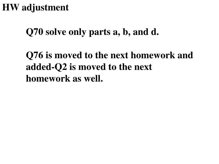
HW adjustment. Q70 solve only parts a, b, and d. Q76 is moved to the next homework and added-Q2 is moved to the next homework as well. The Binomial Distribution. Section 3.4. An experiment is called a binomial experiment if it satisfies the following conditions:.

E N D
HW adjustment Q70 solve only parts a, b, and d. Q76 is moved to the next homework and added-Q2 is moved to the next homework as well.
The Binomial Distribution Section 3.4 An experiment is called a binomial experiment if it satisfies the following conditions: The experiment of interest here consists of a sequence of n sub-experiments called trials, where n is fixed in advance of the experiment. Each trial can result in one of two outcomes usually denoted by success (S) or failure (F). These trials are independent (outcome of one trial doesn’t affect any of the others). The probability of success, p, is constant from trial to trial
The Binomial Distribution Section 3.4 What the above is saying: The experiment consists of a group of nindependent Bernoulli sub-experiments, where n is fixed in advance of the experiment and the probability of a success is p. What we are interested in studying is the number of successes that we may observe in any run of such an experiment.
The Binomial Distribution Section 3.4 The binomial random variable X = the number of successes (S’s) among n Bernoulli trials or sub-experiments. We say X is distributed Binomial with parameters n and p, The pmf can become (depending on the book), The CDF can become (also depending on the book),
The Binomial Distribution Section 3.4 The mean, the variance and the standard deviation:
The Binomial Distribution Section 3.4 When to use the binomial distribution? When we have n independent Bernoulli trials When each Bernoulli trial is formed from a sample n of individuals (parts, animals, …) from a population with replacement. When each Bernoulli trial is formed from a sample of n individuals (parts, animals, …) from a population of size Nwithout replacement if n/N < 5%.
The Binomial Distribution Section 3.4 Example: Ten light bulbs were chosen at random from a batch of 10000 produced by GE. If we know that 100 of these light bulbs are defective, what is the chance that we will observe 2 or more defectives in this sample? If we sample with replacement.
The Binomial Distribution Section 3.4 Example: Ten light bulbs were chosen at random from a batch of 10000 produced by GE. If we know that 100 of these light bulbs are defective, what is the chance that we will observe 2 or more defectives in this sample? If we sample without replacement.
The Binomial Distribution Section 3.4 An experiment is called a binomial experiment if it satisfies the following conditions: The experiment of interest here consists of a sequence of n sub-experiments called trials, where n is fixed in advance of the experiment. Each trial can result in one of two outcomes usually denoted by success (S) or failure (F).
The Binomial Distribution Section 3.4 Identify the sample space (all possible outcomes) S = {SSSSSSSSSS, SSSSSSSSSF, …, , SSSSSSSSSFF, …., FFFFFFFFFF} How many possible outcomes?
The Binomial Distribution Section 3.4 Identify an appropriate random variable that reflects what you are studying (and simple events based on this random variable) Snew= {0, 1, 2, 3, 4, 5, 6, 7, 8, 9, 10}
The Binomial Distribution Section 3.4 Construct the probability distribution associated with the simple events based on the random variable X = 2 => two success! One of those is {SSFFFFFFFF}
The Hypergeometric Section 3.5 The exact distribution of the above example is called the hypergeometric. The hypergeometric random variable X = the number of successes (S’s) among n trials or sub-experiments. We say X is distributed Hypergeometric with parameters N, M and n
The Hypergeometric Section 3.5 The pmf can become (depending on the book), The CDF
The Hypergeometric Section 3.5
The Binomial Distribution Section 3.4 Example: Each component of the following system (machines in a factory) has a 0.1 chance of breaking down. Assuming that none of these components affect the performance of any of the others, construct the associated probability distribution. 0.1 0.1 0.1 0.1 0.1
The Binomial Distribution Section 3.4 The resulting distribution in table format:
The Binomial Distribution Section 3.4 The resulting distribution in table format:
The Binomial Distribution Section 3.4 Mean: Variance: Standard deviation:
The Binomial Distribution Section 3.4 What is the chance that if you go in at any day and observing these components you will find 0.5+/-2*0.67 of them not working? Approximately using Chebyshev’s rule: Exactly from table:
The Binomial Distribution Section 3.4 The resulting distribution in table format:
The Binomial Distribution Section 3.4 A touch on inference: Say that one day we passed by this factory and found that 4 machines (out of the 5) are not working. Should we be alarmed? Or not? Do you think that the model (governed by the parameters n = 5 and p = 0.1) is appropriate to describe this system? Why? Or why not? Can you find a better model (i.e. a better value of the parameters) that fits this observed data?
The Binomial Distribution Section 3.4
The Binomial Distribution Section 3.4
The Binomial Distribution Section 3.4
The Binomial Distribution Section 3.4 So this sample either happened by chance with probability 0.00045, if the model we are using is true, or is best described by a model with p = 0.8. The likelihood of this data under the current model is 0.00045 and under the new model is 0.4096 So, if the p = 0.1 is not known for sure (it usually is not) then, based on our observation, we favor a model with p = 0.8. What kind of implications does this have for the factory?
The Negative Binomial Distribution Section 3.5 An experiment is called a negative binomial experiment if it satisfies the following conditions: The experiment of interest consists of a sequence of sub-experiments (can be infinite) called trials. Each trial can result in one of two outcomes usually denoted by success (S) or failure (F). These trials are independent. The probability of success, p, is constant from trial to trial We stop this experiment when a fixed number, r, of successes occur.
The Negative Binomial Distribution Section 3.5 What the above is saying: The experiment consists of a group of independent Bernoulli sub-experiments, where r (not n), the number of successes we are looking to observe, is fixed in advance of the experiment and the probability of a success is p. What we are interested in studying is the number of failures that precede the rth success. Called negative binomial because instead of fixing the number of trials n we fix the number of successes r.