Download
1 / 18
180 likes | 339 Vues
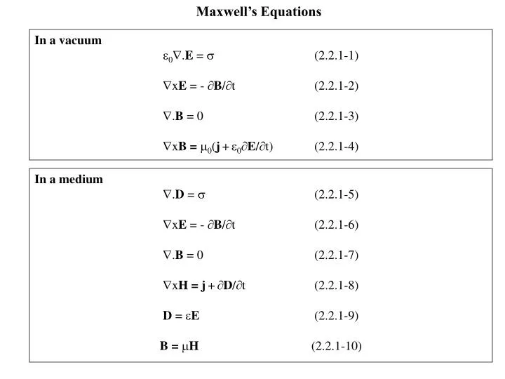
Maxwell’s Equations. In a vacuum 0 . E = (2.2.1-1) x E = - B / t (2.2.1-2) . B = 0 (2.2.1-3) x B = 0 ( j + 0 E / t) (2.2.1-4). In a medium . D = (2.2.1-5) x E = - B / t (2.2.1-6) . B = 0 (2.2.1-7) x H = j + D / t (2.2.1-8)

E N D
Maxwell’s Equations In a vacuum 0.E = (2.2.1-1) xE = - B/t (2.2.1-2) .B = 0 (2.2.1-3) xB = 0(j+0E/t) (2.2.1-4) In a medium .D = (2.2.1-5) xE = - B/t (2.2.1-6) .B = 0 (2.2.1-7) xH = j+D/t (2.2.1-8) D = E (2.2.1-9) B = H (2.2.1-10)
Classical Treatment of Magnetic Materials The ferromagnetic domains, say of a piece of iron, have magnetic moments i giving rise to a bulk magnetization per unit volume M = (1/V) iI (2.2.2-1) This has the same effect as a bound current density jb where jb = xM (2.2.2-2) In the vacuum equation (2.2.1-4) we must include in the j both thebound part, jb and the “free” or externally applied part, jf. (1/0)xB = jb+jf + 0E/t (2.2.2-3) We wish to write this equation (2.2.2-3) in the form xH = jf +0E/t (2.2.2-4) by including jb in the definition of H. This can be done if we let H = (1/0)B – M (2.2.2-5) To get a simple relation between B and H we assume M to be proportional to B or H. M = mH (2.2.2-6) Where the constant mis the magnetic susceptibility. This gives B= 0(1 + m)H (2.2.2-7)
Classical Treatment of Dielectrics The polarization P per unit volume is the sum over all the individual moments p, of the electric dipoles. This gives rise to a bound charge density b = - .P (2.2.3-1) In the vacuum equation (2.2.1-1) we must include both the bound and the free charge; 0.E = f + b (2.2.3-2) We wish to write this in the simple form .D = f (2.2.3-3) by including b in the definition of D. This can be done by letting D = 0E + P = E (2.2.3-4) If P is linearly proportional to E P =0eE (2.2.3-5) Then is a constant given by = (1 + e)0 (2.2.3-6)
The Dielectric Constant of a Plasma From single particle theory, it can be shown that a time-varying E field gives rise to a polarisation current (/B2)E/t, which leads in turn to a corresponding charge density p/t + . jp = 0 (2.2.4-1) From (2.2.1-4) xB = 0(jf +jp + 0E/t) (2.2.4-2) We wish to write this in the form xB = 0(jf + E/t) (2.2.4-3) This can be done if we let = 0 + jp/(E/t) (2.2.4-4) so that = 0 + /B2 or R = /0 = 1 + 0c2/B2 (2.2.4-5) as 00 = 1/c2
Kinetic Theory - Brief Introduction fdv is the number of particles per m3 at position r, and time t with velocity components in the interval v, v + dv. Clearly, if we integrate this in velocity space n(r,t) = ∫f(r,v,t) dv (2.3-1) Note that dv is not a vector but stands for the incremental volume in velocity space. The distribution function can be used to derive averages such as the root mean square velocity n(r,t)vrms = (average v2)0.5 = (∫v2f(r,v,t) dv) 0.5(2.3-2) or average magnitude of velocity n(r,t)(average v) = ∫vf(r,v,t) dv (2.3-3) and the average magnitude of the velocity component in a particular direction for example n(r,t)(average vx) = ∫vxf(r,v,t) dv (2.3-4) For a Maxwellian distribution these quantities are; vrms = (3kBTe/(m))0.5(2.3-5) (average v) = 2(2kBTe/(m))0.5(2.3-6) (average vx) = (2kBTe/(m)) 0.5(2.3-7)
The Boltzmann Equation • The fundamental equation which f has to satisfy is the Boltzmann equation. • ∂f/∂t + v.f + F/m. ∂f/∂v= (∂f/∂t)c(2.3.1-1) • where F is the force acting on the particles and (∂f/∂t)c is the time rate of change of f due to collisions. • The symbol stands for the gradient in ordinary space while ∂/∂v stands for the gradient in velocity • space, so that • ∂/∂v = ux∂/∂vx + uy∂/∂vy + uz∂/∂vz (2.3.1-2) • where ux, uy and uz are unit vectors in the x, y and z directions respectively. The left hand side of • (2.3.1-1) is just the total derivative with respect to time of f(r,v,t) as seen in a frame moving in the • 6-dimesnsional phase space (r,v) with the particles. The Boltzmann equation essentially states that • the for a system of particles, the density in their phase space is altered only by collisions, (∂f/∂t)c. • In a sufficiently hot plasma the collisions can be neglected, and if the force F is entirely electro- • magnetic, then the Boltzmann equation takes on the special form of the Vlasov equation. • ∂f/∂t + v.f + q/m(E + vxB). ∂f/∂v= 0 (2.3.1-3) • Where collisions play a role there are various models for the collision term e.g. when there are collisions with neutral particles (distribution function fn) with a characteristic constant collision time , then one may use the Krook collision term • (∂f/∂t)c. = (fn – f)/ (2.3.1-4) • When the collisions are Coulomb collisions, the Fokker Planck model for the collision term • (∂f/∂t)c. = ∂/∂v. (f<v>)1/2∂2/∂v∂v: (f<vv>) (2.3.1-5) • gives the Fokker- Planck Equation, where v is the change in velocity in a collision.
Derivation of the Fluid Equations • By taking “moments” of the Boltzmann equation (2.3.1-1) on can obtain fluid equations. Taking • moments involves multiplying by some factor e.g. 1, mv, 1/2mvv and integrating over velocity • space (∫(…)dv). • The first moment gives the equation of continuity (which describes the flow of the density n) • ∂n/∂t + .(nu) = 0 (2.3.2-1) • where n is the plasma density and u is average velocity (i.e. fluid velocity). The second moment • gives the equation of motion (which describes the flow of momentum mu) • mn(∂u/∂t + (u.)u) = qn(E + uxB) - .P + Pij (2.3.2-2) • where P is the stress tensor • P = mn(∫fwwdv) (2.3.2-3) • where w is the thermal velocity of a particle i.e. the actual velocity of the particle minus the • average velocity u, and Pij is the moment involving the collision term of species i with species j. • The third moment describes the flow of energy (heat flow equation) and involves a thermal conductivity • tensor (in the same way as the equation of motion involved a stress tensor). The equation of state (p = ) • is a simple form of the heat flow equation.
The Equation of Continuity The conservation of matter requires that the total number of particles N in a volume V can change only if there is a net flux of particles across the surface S bounding that volume. ∂N/∂t = ∫(∂n/∂t)dV = -∫nu.dS (2.4.1) where nu is the particle flux (n is the particle density, u is the representative particle (fluid) velocity) and dS is the outward-pointing element of area of the surface bounding the volume V. Applying the divergence theorem to (2.4.1) -∫nu.dS = -∫.(nu)dV(2.4.2) so that ∂n/∂t + .(nu) = 0(2.4.3) (see equation 2.3.2-1). This is the equation of continuity, and there is one such equation for each species (ions, electrons). Any terms describing sources and sinks have to be explicitly added to this equation.
The Equation of Motion 1/2 • Maxwell’s equations tell us how E and B behave for a given plasma state. However, to solve the • self-consistent problem we need to know how the plasma state evolves given E and B. One of the • equations which do this is the equation of motion (see 2.3.2-2). • mn(∂u/∂t + (u.)u) = qn(E + uxB) - .P + Pij (2.5-1) • Note that this can also be “derived” from the equation of motion of a single, charged particle (charge q) • in fields E and B. • mdv/dt = q(E + vxB) (2.5-2) • The time derivative is to be taken at the position of the particle. If there are no collisions or thermal • motion in a system of a number of such particles, and the average velocity u is the same as the individual particle velocity v, then we can multiply (2.5-2) by n to obtain • mndu/dt = qn(E + vxB) (2.5-3) • However, we wish to have the change of u with respect to a fixed set of space coordinates so that we • have to transform the time derivative (at the position of the particle) of a vector quantity G(r,t) as follows • dG(r,t) /dt = ∂G(r,t)/∂t + dr/dt.G((r,t) (2.5-4) • where d/dt is often referred to as the convective derivative. Note that dr/dt. is a scalar differential • operator. Using (2.5-4) with u as G, equation (2.5-3) becomes (with dr/dt = u, motion with the fluid element) • mn(∂u/∂t + (u.)u) = qn(E + uxB) (2.5-5)
The Equation of Motion 2/2 We could derive (but will not do so here) the additional term (the gradient of the stress tensor) P. For the case where the kinetic distribution is an isotropic Maxwellian, the stress tensor is diagonal with element p (pressure). p 0 0 0 p 0 0 0 p If however, the Maxwellian distribution is non-isotropic with temperatures T and Tin the presence of a magnetic field (in the third component direction) then the elements are p 0 0 0 p 0 0 0 p In an ordinary fluid, the off-diagonal elements are usually associated with viscosity as a result of collisions. This viscosity is characterized by the mean free path of collisions. In a plasma there is a similar effect even in the absence of “traditional” collisions. The Larmor gyration of particles around the magnetic field sets the scale for this “collisionless” viscosity. Collisions for a partially ionised gas, i.e in the presence of neutral gas, can be roughly included as follows. If uois the velocity of the neutral gas, then the momentum lost per collision will be proportional to the relative velocity u - uo. If , the mean free time between collisions is approximately constant, the resulting force can be written as -mn(u - uo)/ . The equation of motion (2.5-1) then becomes mn(∂u/∂t + (u.)u) = qn(E + uxB) - .P - mn(u - uo)/ (2.5-6) This is to be contrasted with the Navier-Stokes equation for ordinary fluids (∂u/∂t + (u.)u) = - p + 2 u (2.5-7) where is the kinematic viscosity coefficient which is just the collisional part of .P - p in the absence of magnetic fields. This equation describes a fluid in which there are frequent collisions between particles.
The Equation of State One more equation is required to close the system of equations and that is the equation of state. It is common to use the thermodynamic equation of state p = C(2.6-1) where C is a constant, and is the ratio of the specific heats (that of constant pressure to that of constant volume). Therefore p/p = / (2.6-2) For isothermal compression p = (nkBT) = kBTn (2.6-3) so that is clearly 1. For adiabatic compression, the temperature changes as well so that will be greater than 1. If N is the number of degrees of freedom involved, then = (2 + N)/N (2.6-4) The validity of the equation of state requires that heat flow is negligible, that is that the thermal conductivity is low. This is more likely to be so perpendicular to B than parallel to it. Most basic phenomena can be described adequately by the crude assumption (2.6-1).
The Complete Set of Fluid Equations • = niqi + neqe • (2.7-1) • j = niqivi + neqe ve • 0.E = niqi + neqe (2.7-2) • xE = - B/t (2.7-3) • .B = 0 (2.7-4) • 1/0(xB) = niqivi + neqe ve+0E/t (2.7-5) • mjnj (∂vj/∂t + (vj.)vj) = qjnj (E + uxB) - pj(2.7-6) • ∂nj/∂t + .(njvj) = 0 (2.7-7) • pj = C jnj(2.7-8) • There are 16 scalar unknowns; nj, ne, pj, pe, vi, ve , E and B,and 18 scalar equations if we count each • vector equation as 3 scalar equations. However, 2 of the Maxwell’s equations are redundant since (2.7-2) and (2.7-4) can be recovered from the divergences of (2.7-3) and (2.7-5). The simultaneous solution of this set of equations gives a self-consistent set of fields and motions of the fluid approximation.
Fluid Drifts Perpendicular to B mn(∂v/∂t + (v.)v) = qn(E + vxB) - p(2.8-1) The ratio of term 1 to term 2 is (mniv)/(qnvB) ≈ /c where is the characteristic frequency of variation, and c is the cyclotron frequency (c.f. single particle motion). For motions slow compared to c and for flows small so that the term (v.)v can be neglected (usually this is checked a posteriori), we have qn(E + vxB) - p= 0(2.8-2) Taking the cross product with B we have v= ExB/B2 - pxB/(qnB2)(2.8-3) The first term on the right hand side of 2.8-3) is referred to as the ExB drift (vE), and the second term on the right hand side is referred to as the diamagnetic drift (vD). Since, for the diamagnetic drift, ions and electrons move in opposite directions, there is a diamagnetic current (assuming ni = ne = n) jD = ne(vDi - vDe)(2.8-4)
Fluid Drifts Parallel to B mn(∂vz/∂t + (v.)vz) = qnEz - ∂p/∂z(2.9-1) We will assume that we can neglect the convective term (v.)vz , so that (with (2.6-2)) ∂vz/∂t = (q/m)Ez – (kBT)/(mn)∂n/∂z (2.9-2) This shows that plasma is accelerated along B under the combined electrostatic (Ez = -∂/∂z) and pressure gradient forces. If this is applied to the “massless” electrons (limit m 0) and q = - e, we have e∂/∂z = (kBT)/n)∂n/∂z (2.9-3) Electrons are so mobile that their heat conductivity is almost infinite. We may then assume isothermal electrons, so that taking = 1 and integrating gives e = kBTeln(n)+ C (2.9-4) or n = n0exp(e/(kBTe)) (2.9-5) This is the Boltmann’s relation for electrons.
The Plasma Resistivity 1/2 The fluid equations of motion for ions and electrons are (2.5-1) mene (∂ve/∂t + (ve.)ve) = -en(E + vexB) - pe ++ . e+ Pei (2.11.1-1) Mini (∂vi/∂t + (vi.)vi) = en(E + vixB) - pi++ . i+ Pie (2.11.1-2) The terms Pei and Pie represent respectively, the momentum gain per unit volume per unit time) of the electron fluid caused by collisions with ions and vice versa. The stress tensor Pj has been split into the isotropic part pj and the anisotropic viscosity tensor j. Like particle collisions which give rise to stresses within each fluid individually, are contained in j. Since these collisions do not give rise to much diffusion we shall neglect this term . j . As for the terms Pei and Pie which represent friction between the two fluids, the conservation of momentum requires Pei = - Pie (2.11.1-3) We can write Pei in terms of the collision frequency ei so that Pei = mene(vi - ve)ei (2.11.1-4) and similarly for Pie, Since the collisions are Coulomb collisions one would expect Peii to be proportional to the Coulomb force which is proportional to e2 (for singly charged ions). Furthermore Peii must be proportional to the density of electrons, ne and to the density of scattering centres ni. Finally Peii should be proportional to the relative velocity of the two fluids. Pei = n2e2(vi - ve) (2.11.1-5) where is a constant of proportionality (and the plasma approximation ne = ni . has been used). This constant is the specific resistivity as will be demonstrated below.
The Plasma Resistivity 2/2 • ei = n2e2/(me) (2.11.1-6) • ei = nee4/(1602me2v3) (2.11.1-7) so that (when we replace v2 by (kBTe/me) • = e2me0.5/((40)2(kBTe)1.5) (2.11.1-8) • This expression is correct for large angle collisions but because of the long range of the Coulomb collisions, small angle collision are much more frequent and the cumulative effect of such collisions leads to a modification of the result (2.11.1-8) as shown by Spitzer (1952) in that a multiplicative factor to the right hand side of , (2.11.1-8), ln, is required. (which represents the maximum (normalized) impact parameter), for singly charged ions is, • = 3/(2e3)((kB2Te3)/(ne)0.5 (2.11.1-9) • and this makes ln a very slowly varying function of ne and Te. • The Physical meaning of • Let us suppose an electric field exists in the plasma and the current that drives it is carried entirely by the electrons which are much more mobile than the electrons. Let B = 0, and kBTe = 0 so that .Pe = 0 thenthe steady-state electron equation of motion (2.11.1-1) reduces to • ene E = Pei (2.11.2-1) • Since the current density j is en(vi - ve)) then Pei can be written as • Pei = nej (2.11.2-2) • so that (2.11.2-1) becomes • E = j (2.11.2-3)
The Single Fluid MHD Equations 1/2 For a quasi-neutral plasma composed of singly-charged ions and electrons we define a mass density , a mass velocity v and a current density j = (mene + Mini) n(me + Mi) (2.12-1) v = (1/)(Minivi + meneve) (Mivi + meve)/(me + Mi) (2.12-2) j = e(nivi - neve) ne(vi - ve) (2.12-3) In the equations of motion (2.11-1) and (2.11-2) we will neglect the (v.)v and . terms, assume ni = ne, = n, and add a gravitational force term (mng) to represent any non-electromagnetic force applied to plasma. men∂ve/∂t = - en(E + vexB) - pe ++ meng + Pei (2.12-4) Min ∂vi/∂t + = en(E + vixB) - pi+ Meng + Pie (2.12-5) If we add equations (2.12-4) and (2.12-5) and use the definitions (2.12-1) to (2.12-3) we have (with total pressure p = pi + pe) ∂v/∂t = jxB - p+ g (2.12-6) This is the single fluid equation of motion describing mass flow. Now multiply (2.12-4) by Mi and (2.12-5) by me,and subtract the former from the latter, we have Mimen∂(vi–ve)/∂t = en(Mi + me)E + en(Mivi + meve)xB + Mipe - mepi - (Mi + me) Pei (2.12-7) With the help of (2.12-1) to (2.12-3) this becomes Mimen∂(j/n)/∂t = eE - (Mi + me)nej - mepi + Mipe + en(Mivi + meve)xB (2.12.8) The last term can be simplified to be (/n)v – (Mi - me)j/(ne) so that dividing 2.12-7) by e we have E + vxB = j + 1/(ne)(jxB -pe)(2.12.9) where the ∂(j/n)/∂t term has been neglected (for slow motions) and limit of small me/Mi has been applied. This equation is called the generalised Ohm’s Law. The jxB term is called the Hall current term and often the last term in this equation is small enough to be neglected.
The Single Fluid MHD Equations 2/2 Now equations of continuity for mass density , and charge density (see (2.7-1)) can be obtained by combining the electron and ion continuity equations so that the MHD set of equations is ∂v/∂t = jxB - p+ g (2.12-10) E + vxB = j (2.12-11) ∂∂t + .(v) = 0 (2.12-12) ∂∂t + .j = 0 (2.12-12) Together with Maxwell’s equations these are often used to describe the equilibrium state of the plasma. They are less accurate than the two-fluid equations for use in describing wave motion. For problems involving resistivity their relative simplicity mostly outweighs their disadvantages. These equations have been used extensively by astrophysicists working in cosmic electrodynamics, and by people working on MHD energy conversion, and by fusion theorists.