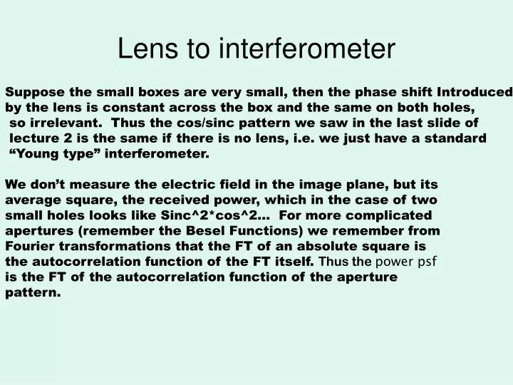
1. Lens to interferometer Suppose the small boxes are very small, then the phase shift Introduced by the lens is constant across the box and the same on both holes, so irrelevant. Thus the cos/sinc pattern we saw in the last slide of lecture 2 is the same if there is no lens, i.e. we just have a standard “Young type” interferometer. We don’t measure the electric field in the image plane, but its average square, the received power, which in the case of two small holes looks like Sinc^2*cos^2… For more complicated apertures (remember the Besel Functions) we remember from Fourier transformations that the FT of an absolute square is the autocorrelation function of the FT itself. Thus the power psf is the FT of the autocorrelation function of the aperture pattern.

2. Power versus correlation Up until now we have assumed that our detection equipment measures the total light power received in the image plane. In other words I(p) = <E(p)E*(p)> Where f is the phase angle between E1 and E2. The high resolution part of this signal is the last term which oscillates like cos (kpDX/f) while the first two terms represent the total power coming through the 1st and 2nd slits. These may contain very large terms due to sky radiation that have nothing to do with the target, so it would be nice to get rid of them. We can do this if we have a Correlator rather than a detector. A correlator measures the average produce of two signals: I’ll describe later how some correlators work.

3. Correlation So now we can abstract our optical system even further , throw away the focal system behind the aperture and replace it with a correlator. Then, if I have two small slits looking at a point source, then the correlated flux is: Where D is the Optical Path Delay(OPD), the difference in path length from the source to slit 2 versus slit 1. If the two “slits” are separated by a baseline vector B, and the source is in the direction n, then: or: • is the angle between the baseline and the source. Note that C does not depend on the position of the receivers on the ground but only on their separation vector.

4. Correlation Now let’s consider what happens if we have more than one source of radiation on the sky. Then antenna 1 receives not only electric field E1 from one source but also, say, F1 from the other source, with similar E2 and F2 at the other receiver. Then the formulas for I and C should contain complicated terms like: reflecting the difference in position between the two sources. This would be very messy, but fortunately astronomical sources are incoherent, that is, the phase difference between two unrelated sources is never completely constant, but drifts quickly or slowly with time (to be described later). So a term like actually shows up as where J is a random number and so the cos averages to zero and can be ignored. This would not be true if there were coherent sources (like lasers) distributed over the sky.

5. Correlation So, surprisingly or not, if I have a complicated source on the sky, the response of the interferometer is determined by the sum of the intensities from the individual components rather than the electric fields. Symbolically: Where is the emitted intensity as a function of the spatial position. This looks sort of like a Fourier Transform but not quite. The term is non-linear in the position n on the sky because of the complicated spherical trigonometry. But in a small piece of sky near some reference point Lo this can be linearized: is the interferometric delay as a function of position in the field, L is the vector position relative to Lo. (U,V) are the “UV” coordinates of the baseline and equal the physical vector baseline projected onto the sky at Lo. For narrow band (e.g. radio) measurements the wavenumber is included in the definition of U.

6. If we are smart enough to design a fully complex correlator, that also measures then we can write more directly: which looks exactly like a fourier transform. The easiest way to get the imaginary part of the correlation is to insert a quarter wave (l/4) extra delay in the path, although this can be tricky for a wide band system. Ideally this would be all there is to interferometry: if you measure a whole lot of baselines you get an estimate of C over a complete piece of the UV-plane, and by a simple numerical Fourier Transform you can reconstruct I(L). This is called Aperture Synthesis. The goal of measuring many UV points is partly achieved by sitting down and letting the rotation of the Earth change the projection of the baseline on the sky, and partly by having many telescopes at different positions to form into pairs, or moving around the telescopes you have.